We often replace specific text values with other text values. In such scenarios, the SUBSTITUTE function appears very handy. In this article, I’ll demonstrate 7 ideal examples of how to use the SUBSTITUTE function in Google Sheets. Also, I’ll discuss 2 alternatives to the SUBSTITUTE function in Google Sheets.
A Sample of Practice Spreadsheet
You can copy our practice spreadsheets by clicking on the following link. The spreadsheets contain an overview of the datasheet and an outline of the described examples to use the SUBSTITUTE function in Google Sheets.
What Is SUBSTITUTE Function in Google Sheets?
The SUBSTITUTE function is a text function in Google Sheets that can replace any existing string with a new string.
Syntax
The syntax of the SUBSTITUTE function is as follows:
SUBSTITUTE(text_to_search, search_for, replace_with, [occurrence_number])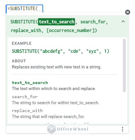
Argument
The arguments of the SUBSTITUTE function are the following:
| Argument | Requirement | Function |
|---|---|---|
| text_to_search | Required | The text where text substitution occurs. |
| search_for | Required | The string to be substituted. |
| replace_with | Required | The string that will substitute the existing string. |
| [occurrence_number] | Optional | The instance of the string to be substituted. |
Output
The formula SUBSTITUTE(“L. Messi”, “L.”, “Lionel”) will show Lionel Messi as output.
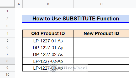
7 Ideal Examples to Use SUBSTITUTE Function in Google Sheets
First, let’s get used to our dataset. The dataset contains several old product IDs for an electronics shop. We’ll use the SUBSTITUTE function to replace these old product IDs with new product IDs according to various formats.
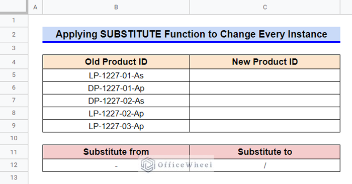
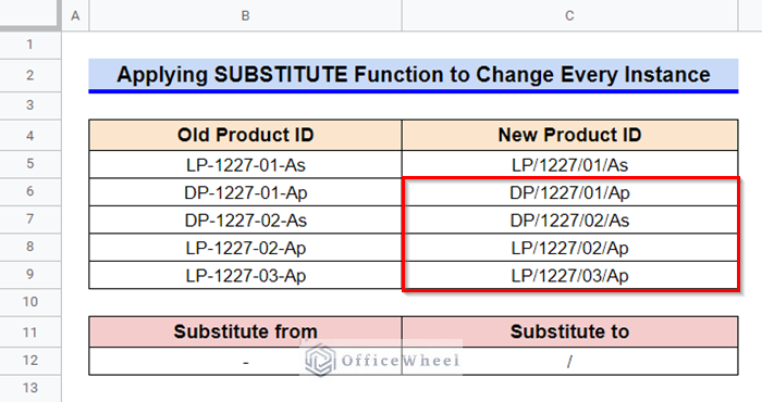
1. Applying SUBSTITUTE Function to Change Every Instance
While using the SUBSTITUTE function, if we don’t provide the optional argument (i.e. occurrence_number), then the SUBSTITUTE function replaces all occurrences. Let’s replace all the Hyphen (-) symbols with the Slash (/) symbol in our dataset.
Steps:
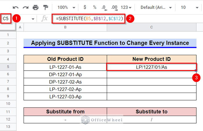
- First, select Cell C5.
- After that, type in the following formula-
=SUBSTITUTE(B5,$B$12,$C$12)- After that, press the Enter key to get the required value.
- To make the Fill Handle icon visible, hover your mouse pointer above the right-bottom corner of Cell C5.
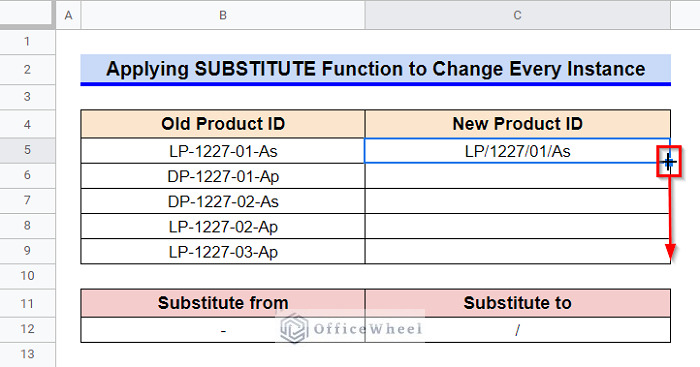
- Finally, use the Fill Handle icon to copy the formula to other cells of Column C.
Read More: How to Remove Everything after Character in Google Sheets
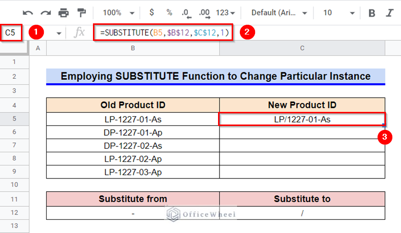
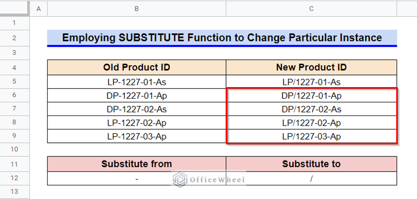
2. Employing SUBSTITUTE Function to Change Particular Instance
Now, let’s provide the occurrence_number argument to the SUBSTITUTE function. We’ll change only the first instance of the Hyphen (-) symbol with Slash (/) symbol this time.
Steps:
- Select Cell C5 and type in the following formula-
=SUBSTITUTE(B5,$B$12,$C$12,1)- Then, press the Enter key to get the required output.
- Finally, use the Fill Handle icon to copy the formula in other cells.
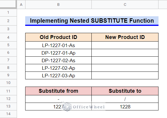
3. Implementing Nested SUBSTITUTE Function
If we require more than one change in a single cell, we can implement a nested SUBSTITUTE function to achieve our desired result. For this example, we’ll make the following two changes in our dataset. Now let’s apply a nested SUBSTITUTE function to implement the desired change.
Steps:
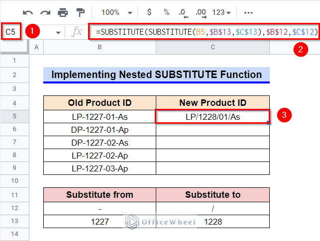
- To start, select Cell C5 first.
- Afterward, type in the following formula-
=SUBSTITUTE(SUBSTITUTE(B5,$B$13,$C$13),$B$12,$C$12)- Next, press Enter key to get desired output.
Formula Breakdown
- SUBSTITUTE(B5,$B$13,$C$13)
First, this SUBSTITUTE function replaces elements of Cell B13 (1227) with elements of Cell C13 (1228) in the string of Cell B5.
- SUBSTITUTE(SUBSTITUTE(B5,$B$13,$C$13),$B$12,$C$12)
The output of the inner SUBSTITUTE function works as the text_to_search for the outer SUBSTITUTE function. After that, the outer SUBSTITUTE function changes all the Hyphen (-) symbols (element in Cell B12) with the Slash (/) symbol (element in Cell C12).
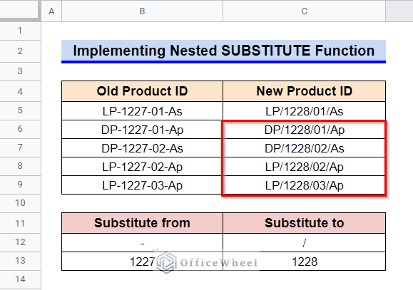
- Now, finally, use the Fill Handle icon to copy the formula to other cells.
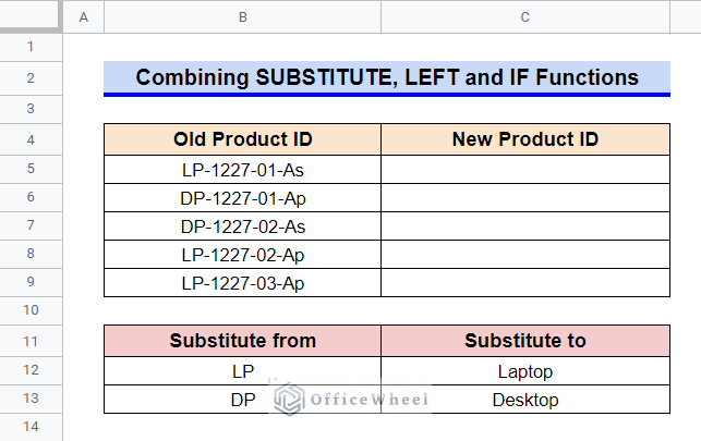
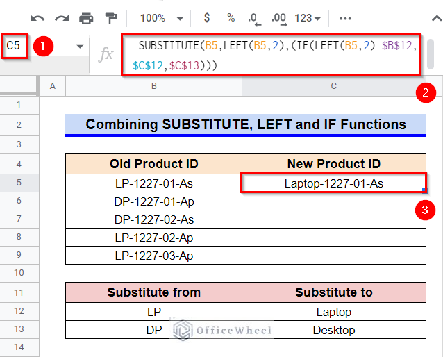
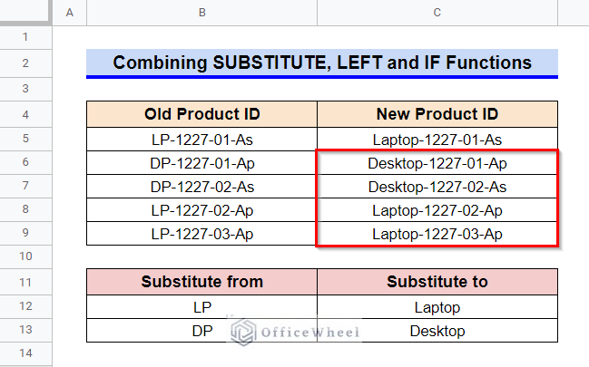
4. Combining SUBSTITUTE, LEFT, and IF Functions for Multiple Characters
If you need to replace multiple characters from the left or right side of the strings in a data range, then you can combine the SUBSTITUTE and IF functions with LEFT or RIGHT functions according to the requirement. For this example, we’ll change 2 characters from the left side of the strings in our data range in the following manner.
Steps:
- First, select Cell C5 and then type in the following formula-
=SUBSTITUTE(B5,LEFT(B5,2),(IF(LEFT(B5,2)=$B$12,$C$12,$C$13)))- After that, press the Enter key next to get the required result.
Formula Breakdown
- LEFT(B5,2)
The LEFT function is used twice in our formula. In both instances, it returns the left 2 characters of the string in Cell B5.
- IF(LEFT(B5,2)=$B$12,$C$12,$C$13)
Then, the IF function checks whether the left 2 characters of the string in Cell B5 match the content of Cell B12. If a match is found then the IF function returns the content of Cell C12. Else, it returns the content of Cell C13.
- SUBSTITUTE(B5, LEFT(B5,2),(IF(LEFT(B5,2)=$B$12,$C$12,$C$13)))
Finally, the SUBSTITUTE function replaces the left 2 characters of the string in Cell B5 with the output returned by the IF function. Note that, you must keep the IF function in a set of parentheses, otherwise the formula won’t execute.
- Finally, use the Fill Handle icon to copy the formula in the other cells of Column C.
Read More: How to Use RIGHT Function in Google Sheets (6 Suitable Examples)
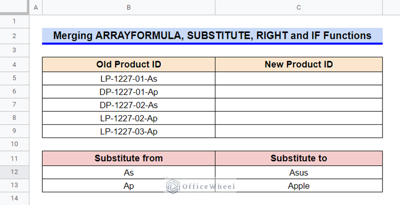
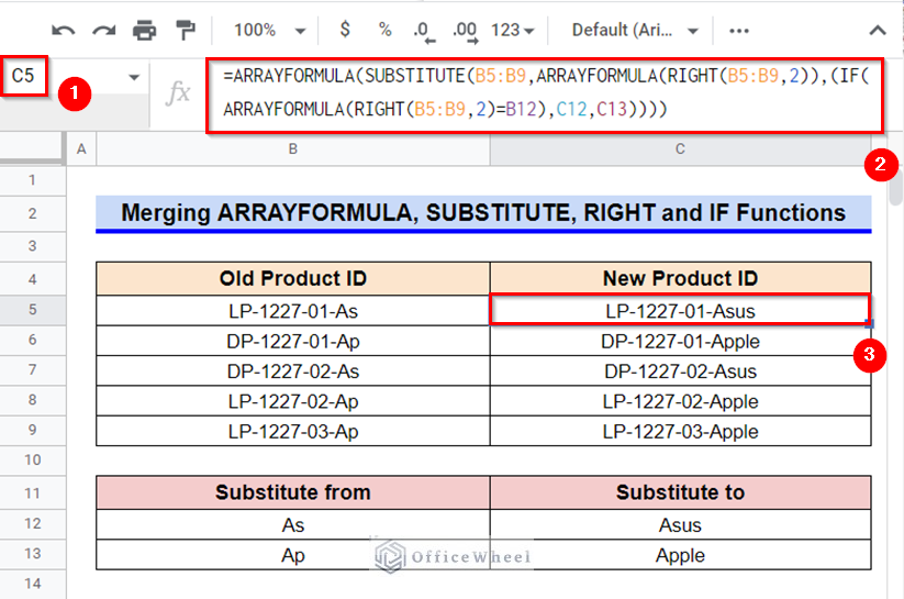
5. Merging ARRAYFORMULA, SUBSTITUTE, RIGHT, and IF Functions for Multiple Characters
Instead of using the Fill Handle icon to copy our formula in other cells, we can use the ARRAYFORMULA function to perform a similar operation for a range. Let’s combine the ARRAYFORMULA function with SUBSTITUTE and IF functions, and instead of the LEFT function, use the RIGHT function to change characters from the right side this time.
Steps:
- Select Cell C5 first.
- Afterward, type in the following formula-
=ARRAYFORMULA(SUBSTITUTE(B5:B9,ARRAYFORMULA(RIGHT(B5:B9,2)),(IF(ARRAYFORMULA(RIGHT(B5:B9,2)=B12),C12,C13))))- Next, press the Enter key to get desired output.
Formula Breakdown
- RIGHT(B5:B9,2)
The RIGHT function is used twice in our formula. In both instances, it returns 2 characters from the right side of the strings in array B5:B9.
- ARRAYFORMULA(RIGHT(B5:B9,2))
This ARRAYFORMULA function helps the non-array function RIGHT to deal with an array.
- IF(ARRAYFORMULA(RIGHT(B5:B9,2)=B12), C12, C13))
Now, the IF function checks whether the 2 rightmost characters of the strings in range B5:B9 match with the content of Cell B12. If a match is found then the IF function returns the content of Cell C12. Else, it returns the content of Cell C13.
- SUBSTITUTE(B5:B9,ARRAYFORMULA(RIGHT(B5:B9,2)),(IF(ARRAYFORMULA(RIGHT(B5:B9,2)=B12),C12,C13)))
Afterward, the SUBSTITUTE function replaces the 2 rightmost characters of the strings in range B5:B9 with the output returned by the subsequent IF function.
- ARRAYFORMULA(SUBSTITUTE(B5:B9,ARRAYFORMULA(RIGHT(B5:B9,2)),(IF(ARRAYFORMULA(RIGHT(B5:B9,2)=B12),C12,C13))))
Finally, this ARRAYFORMULA function helps the non-array function SUBSTITUTE to deal with an array.
Read More: How to Remove Text after Character in Google Sheets (5 Methods)
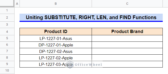
6. Uniting SUBSTITUTE, RIGHT, LEN, and FIND Functions to Retrieve Specific String
We can also use the SUBSTITUTE function united with the RIGHT, LEN, and FIND functions to retrieve a specific string from a longer string. For example, let’s retrieve the brand names from the product IDs for the following dataset. Note that, the brand names don’t have equal string lengths. Hence, using only the RIGHT function won’t help.
Steps:
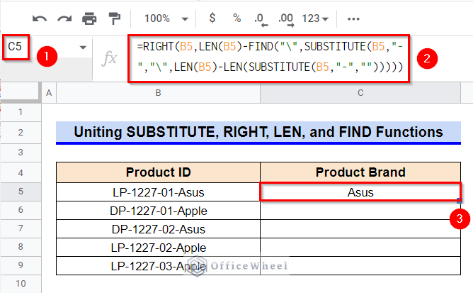
- Select Cell C5 first.
- After that, type in the following formula-
=RIGHT(B5,LEN(B5)-FIND("\",SUBSTITUTE(B5,"-","\",LEN(B5)-LEN(SUBSTITUTE(B5,"-","")))))- Then press the Enter key to retrieve the required string.
Formula Breakdown
- LEN(B5)
The LEN function returns the length of the string in Cell B5. The output here is 15.
- SUBSTITUTE(B5,”-“,””)
The SUBSTITUTE function replaces all the Hyphen (-) symbols from the string in Cell B5. The output here is LP122701Asus.
- LEN(SUBSTITUTE(B5,”-“,””))
Then, this LEN function returns the length of the string returned by the SUBSTITUTE function. The output here is 12.
- LEN(B5)-LEN(SUBSTITUTE(B5,”-“,””))
This part of the formula subtracts the length of the string in Cell B5 and the length of the string returned by the SUBSTITUTE function. The output here is 3. This number indicates the number of Hyphen (-) symbols in the string of Cell B5.
- SUBSTITUTE(B5,”-“,”\”,LEN(B5)-LEN(SUBSTITUTE(B5,”-“,””)))
Since we want to retrieve the string after the last Hyphen (-) symbol, we have substituted the last Hyphen (-) symbol with a Backslash (\) symbol using the SUBSTITUTE function. The output here is LP-1227-01\Asus.
- FIND(“\”,SUBSTITUTE(B5,”-“,”\”,LEN(B5)-LEN(SUBSTITUTE(B5,”-“,””))))
Afterward, the FIND function returns the position of the Backslash (\) symbol in the string LP-1227-01\Asus. The output here is 11.
- LEN(B5)-FIND(“\”,SUBSTITUTE(B5,”-“,”\”,LEN(B5)-LEN(SUBSTITUTE(B5,”-“,””))))
Another subtraction operation is executed by this part of the formula to specify the string length of the brand name. Here, the output is 4.
- RIGHT(B5,LEN(B5)-FIND(“\”,SUBSTITUTE(B5,”-“,”\”,LEN(B5)-LEN(SUBSTITUTE(B5,”-“,””)))))
Finally, the RIGHT function returns the last 4 characters (i.e. the Product Brand name) from the string in Cell B5. The output here is Asus.
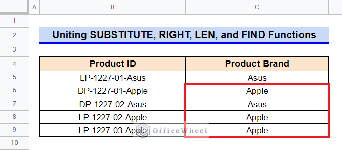
- Finally, use the Fill Handle icon to copy the formula in the other cells of Column C.
Read More: How to Use FIND Function in Google Sheets (5 Useful Examples)
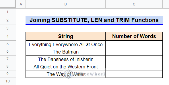
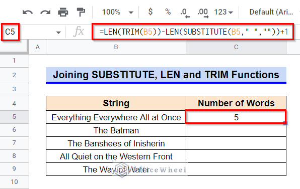
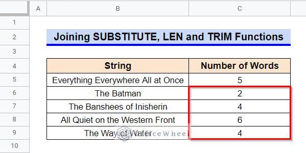
7. Joining SUBSTITUTE, LEN, and TRIM Functions to Count Words
The SUBSTITUTE function can also count the number of words in a string when it is joined with the LEN and TRIM functions. To demonstrate an example of this scenario, we require a new dataset like the following. Now let’s count the number of words in these strings.
Steps:
- To start, select Cell C5 first.
- Afterward, type in the following formula-
=LEN(TRIM(B5))-LEN(SUBSTITUTE(B5," ",""))+1- Next, press Enter key to copy the formula into other cells.
Formula Breakdown
- TRIM(B5)
First, the TRIM function removes all the leading, trailing, or repeated spaces if present in the string of Cell B5.
- LEN(TRIM(B5))
Then, the first LEN function returns the trimmed length of the string in Cell B5.
- SUBSTITUTE(B5,” “,””))
Next, the SUBSTITUTE function replaces all the spaces between the words in the string of Cell B5.
- LEN(SUBSTITUTE(B5,” “,””))
After that, the second LEN function returns the length of the substituted string.
- LEN(TRIM(B5))-LEN(SUBSTITUTE(B5,” “,””))+1
Finally, the subtraction of the two TRIM functions specifies the number of spaces present in the string in Cell B5. A value of 1 is added to that number to get the word count.
- Finally, use the Fill Handle icon, to copy the formula in other cells of Column C.
Read More: How to Remove Last Character from String in Google Sheets
Alternatives to SUBSTITUTE Function in Google Sheets
There are a few alternatives to the SUBSTITUTE function in Google Sheets. Here, we’ll discuss two such alternatives.
1. Utilizing Find and Replace Tool
We can achieve the output of the SUBSTITUTE function even without applying a formula by using the Find and Replace tool from the Edit ribbon in Google Sheets. But the limitation is it can replace only the duplicates of one string at a time.
Steps:
- First, select the range B5:B9.
- Afterward, use the keyboard shortcut CTRL+C to copy the range.
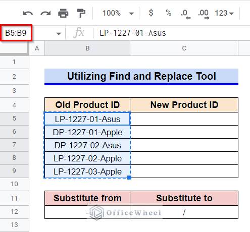
- After that, select Cell C5 and then use the keyboard shortcut CTRL+V to paste the range.
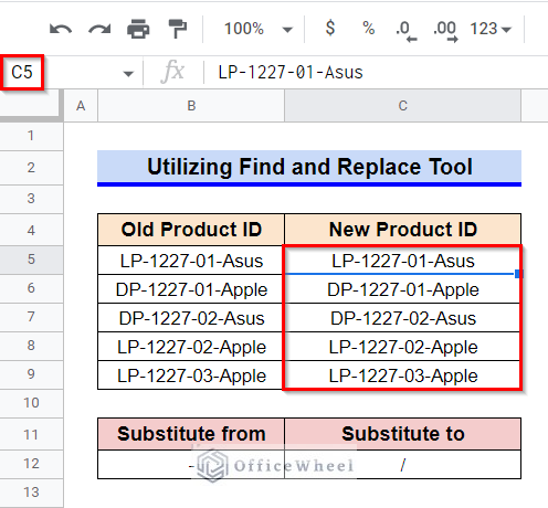
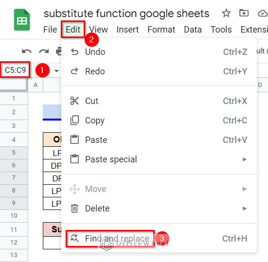
- Now, select the range C5:C9 and then go to the Edit Select Find and Replace tool from the options.
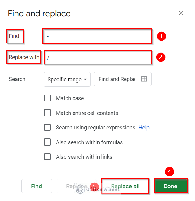
- A window like the following will pop up. Then, in the Find option, enter a Hyphen (-) symbol, and in the Replace with option, enter a Slash (/) symbol.
- Now, click on the Replace All option first and the Done option after that.
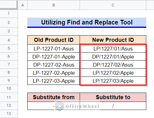
- This will make the desired changes to the range.
Read More: How to Format Date with Formula in Google Sheets (3 Easy Ways)
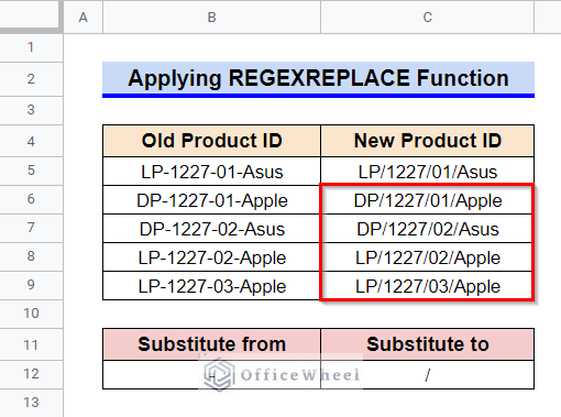
2. Applying REGEXREPLACE Function
The REGEXREPLACE function can also replace strings. However, unlike the SUBSTITUTE function, the REGEXREPLACE function can not replace particular instances.
Steps:
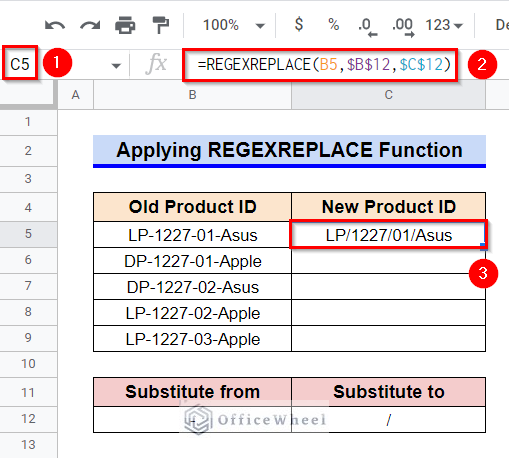
- Select Cell C5 first and then type in the following formula-
=REGEXREPLACE(B5,$B$12,$C$12)- After that, press the Enter key to get the desired changes.
- Finally, use the Fill Handle icon to copy the formula in the other cells of Column C.
How to Substitute Formula with Value in Google Sheets
Sometimes, we require to substitute a formula with value in our worksheets. For example, consider the following dataset where have used the SUBSTITUTE function to change strings. Now, let’s discuss a simple method that can substitute these formulas with values. No function can accomplish this, only the Paste Special command/shortcut can do this.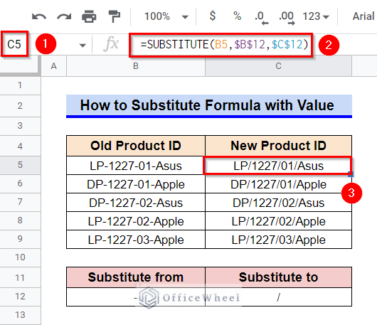
Steps:
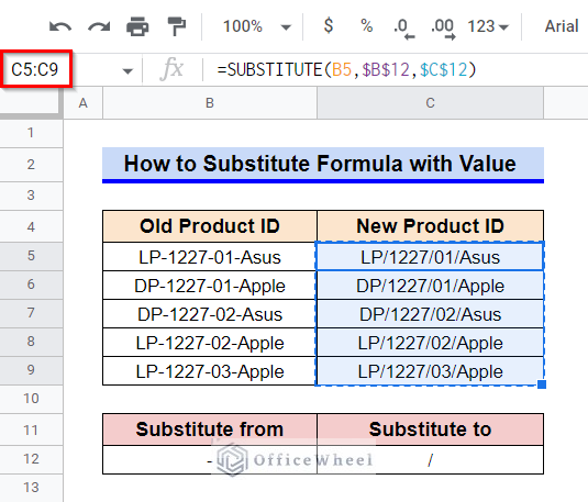
- First, select the range C5:C9.
- Then, use the keyboard shortcut CTRL+C to copy the range.
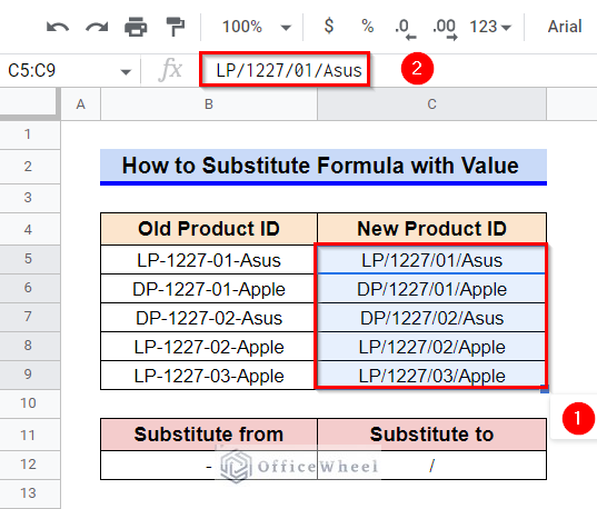
- Now, select Cell C5 and then use the keyboard shortcut CTRL+SHIFT+V to paste the range as a value.
- Thus you can substitute a formula with value.
Read More: Remove Everything after Character Using Google Sheets Formula
Things to Be Considered
- If we don’t enter the occurrence_number argument, then the SUBSTITUTE function will replace every instance of the text to be replaced.
- While substituting multiple characters, we must keep the IF function in a set of parentheses.
Conclusion
This concludes our article to learn how to use the SUBSTITUTE function in Google Sheets. I hope the demonstrated examples were sufficient for your requirements. Feel free to leave your thoughts on the article in the comment box. Visit our website OfficeWheel.com for more helpful articles.
Related Articles
- How to Use SEARCH Function in Google Sheets (5 Examples)
- Remove Characters from a String in Google Sheets (6 Easy Examples)
- Google Sheets Smart Fill: Recognize and Autocomplete Patterns (A Complete Guide)
- How to Remove First Character in Google Sheets
- Convert Text to Date in Google Sheets (3 Easy Ways)