The AVERAGEIF function is basically a combination of the AVERAGE and IF functions. This function is used for returning the average of a range following a single criterion. In this article, I’ll be demonstrating 6 helpful examples of how to use the AVERAGEIF function in Google Sheets.
A Sample of Practice Spreadsheet
You can copy our practice spreadsheets by clicking on the following link. The spreadsheets contain an overview of the datasheet and an outline of the described ways of how to use the AVERAGEIF function in Google Sheets.
What Is AVERAGEIF Function in Google Sheets?
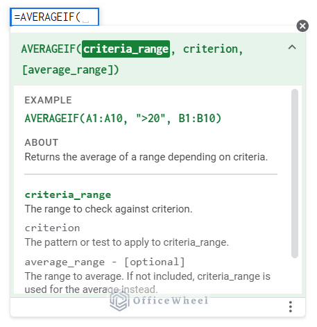
The AVERAGEIF function returns the average of any range specified by a single criterion from any range.
Syntax
The syntax of the AVERAGEIF function is the following:
AVERAGEIF(criteria_range, criterion, [average_range])Argument
The arguments of the AVERAGEIF function are-
| Argument | Requirement | Function |
|---|---|---|
| criteria_range | Required | The range that will be checked for entered criterion. |
| criterion | Required | The condition that will be applied to criteria_range. |
| average_range | Optional | The range you want to average. |
Output
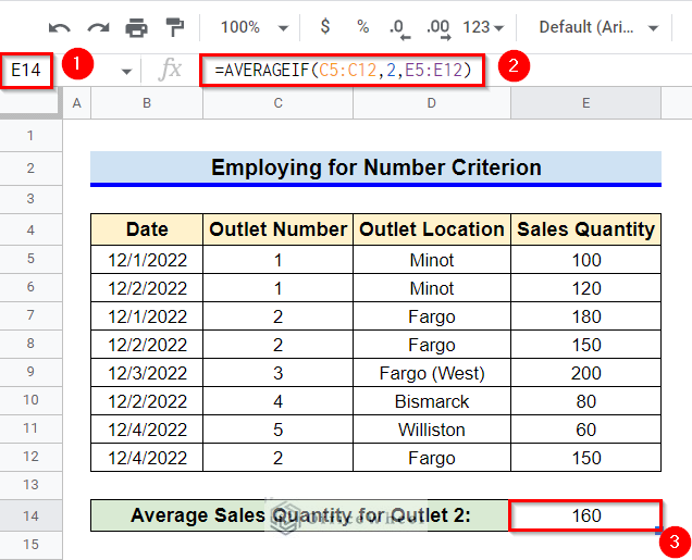
The formula =AVERAGEIF(C5:C12, 2, E5:E12) first searches for a value of 2 in criteria_range C5:C12 and then returns the average of subsequent cells from range E5:E12, where the criterion matches. However, if no match is found, then the formula returns a division by 0 error.
6 Helpful Examples to Use AVERAGEIF Function in Google Sheets
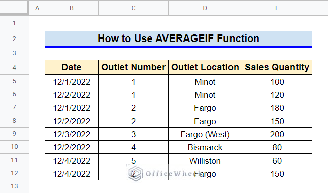
First, let’s get familiar with our datasheet. It contains the sales quantity of several outlets from various locations for different dates. We’ll calculate sales quantity for various criteria from this datasheet. Keep reading to learn how.
Example 1: Apply for Text Criterion
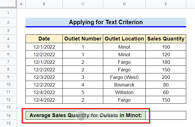
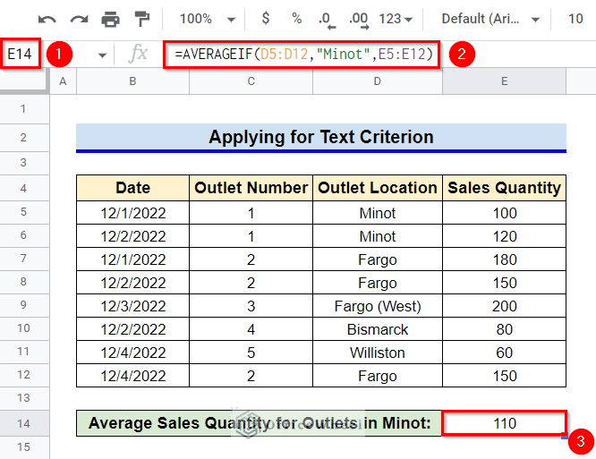
Here, we’ll provide text values as a criterion to apply the AVERAGEIF function in Google Sheets. For example, let’s assume we’ll calculate the average sales quantity for outlets in Minot.
Steps:
- First, select Cell E14.
- After that, type in the following formula-
=AVERAGEIF(D5:D12, "Minot", E5:E12)- Finally, press the Enter key to get the required average value.
Example 2: Employ for Number Criterion
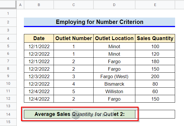
We can also provide numbers as a criterion while employing the AVERAGEIF function. For example, let’s assume we want to find the average sales quantity for outlet 2.
Steps:
- First, select Cell E14.
- Now, type in the following formula in Cell E14–
=AVERAGEIF(C5:C12, 2, E5:E12)- Finally, press the Enter key to get the required result.
Example 3: Implement for Date Criterion
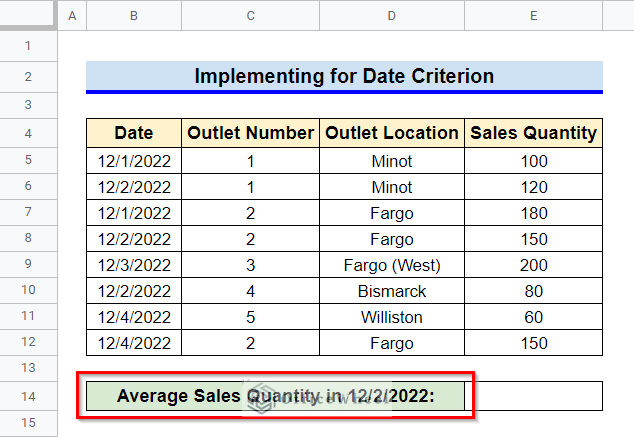
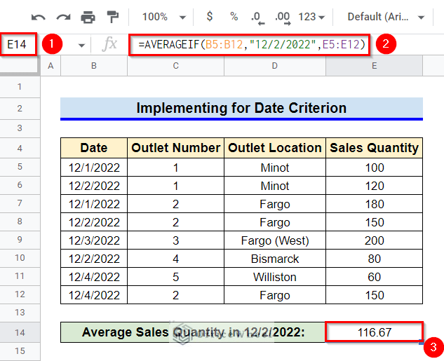
We often need to find the average of different values for specific dates. While implementing the AVERAGEIF function, you can also provide dates as a criterion. For example, let’s consider finding the average sales quantity for 12/2/2022.
Steps:
- Select the cell where you want to calculate the average (Cell E14).
- Now, type in the following formula-
=AVERAGEIF(B5:B12, "12/2/2022", E5:E12)- Finally, press Enter key to get the required value of the average.
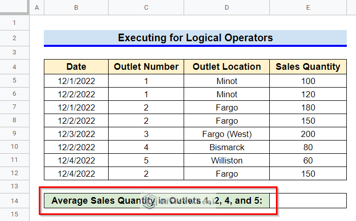
Example 4: Execute for Logical Operators
Logical operators are symbols or words that connect two or more expressions. For example, some of the common logical operators are: Equal to (=), Not equal to (<>), Less than (<), Greater than (>), Less than or Equal to (<=), Greater than or Equal to (>=), etc.
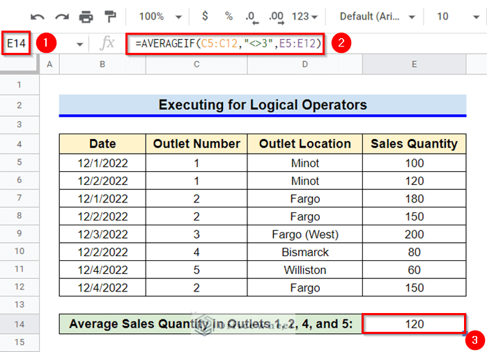
Now, on this occasion, let’s assume we want to find average sales for all the outlets except outlet 3. For this, we can use the “Not equal to” operator.
Steps:
- First, select Cell E14.
- After that, type in the following formula-
=AVERAGEIF(C5:C12,"<>3",E5:E12)- Finally, press Enter key to get the required result.
Example 5: Use for Wildcard Characters
Wildcard characters can help us to find similar strings while applying a set of criteria to any range. The wildcard characters used in Google Sheets are: The asterisk (*), which is used for finding a number of characters, The question mark (?), which is used for finding a single character and The tilde (~), used before “*” or “?” if these characters are not used as wildcard characters.
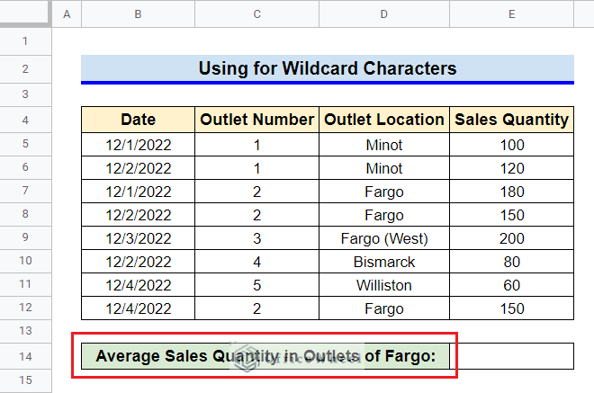
Now, on this occasion, let’s assume we want to calculate the average sales quantity for outlets in Fargo including Fargo (West). We don’t have to use multiple AVERAGEIF functions if we use wildcard characters here.
Steps:
- First, Select Cell E14
- Now, type in the following formula-
=AVERAGEIF(D5:D12,"Fargo*",E5:E12)- Finally, press Enter key to get the required value average value.
Read More: [Fixed!] Wildcard Is Not Working in Google Sheets (5 Solutions)
Example 6: Apply Without Average Range
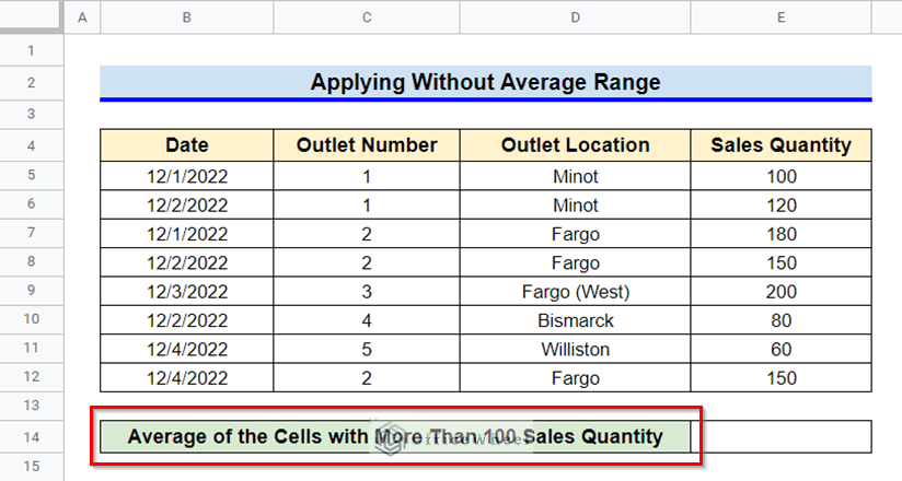
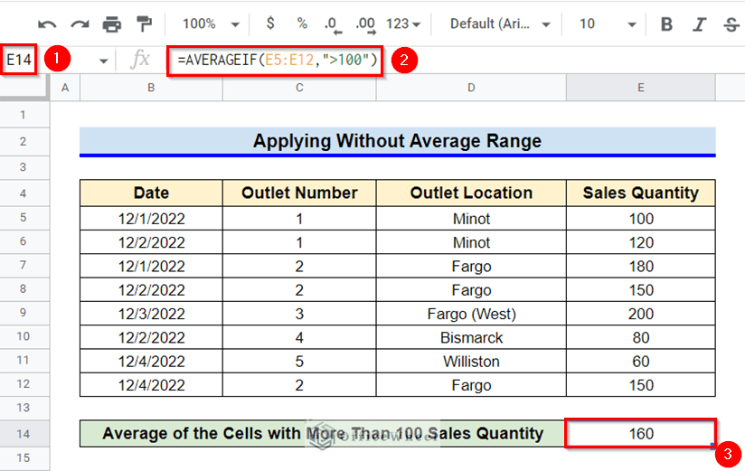
Since the average_range argument is optional, therefore we can skip it if we want. However, if we apply the AVERAGEIFS function without a range to average, the AVERAGEIFS function calculates the average for the criteria_range argument instead.
Steps:
- Select Cell E14 first.
- Afterward, type in the following formula:
=AVERAGEIF(E5:E12,">100")- Finally, press Enter key to return the average for provided criteria range.
Read More: How to Average If Cell Is Not Blank in Google Sheets (5 Ways)
How to Use AVERAGEIF Function for Multiple Criteria in Google Sheets
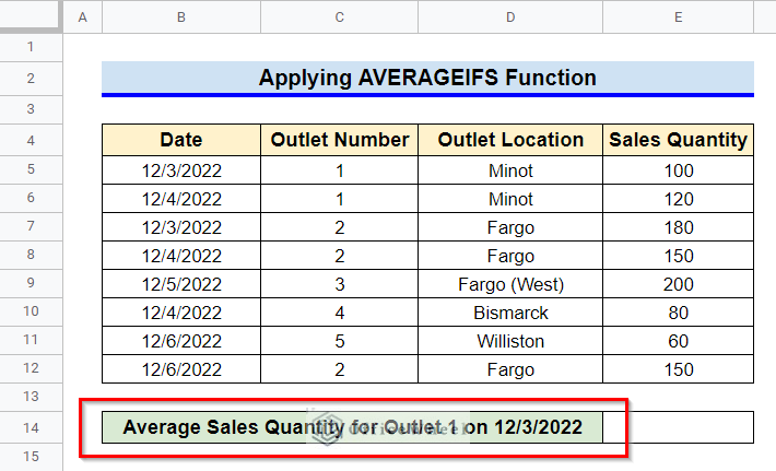
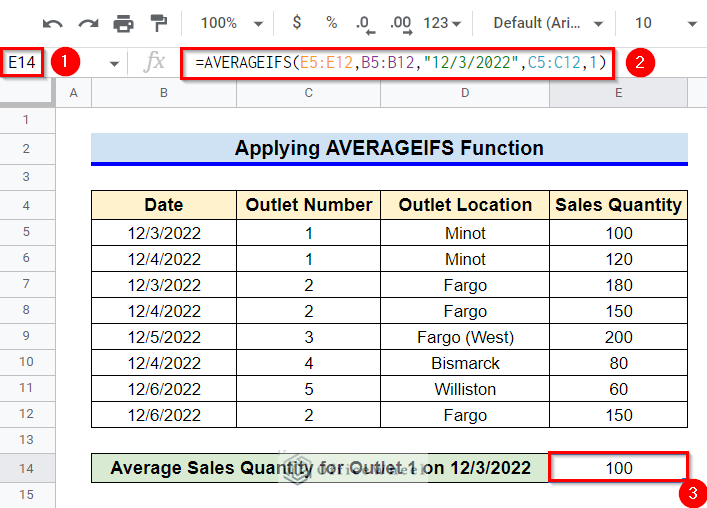
Since the AVERAGEIF function can deal with only a single criterion, you can’t use this function for multiple criteria. However, instead, you can apply the AVERAGEIFS function. For example, let’s calculate the average sales quantity for outlet 1 on 12/3/2022.
Steps:
- First, select Cell E14.
- After that, type in the following formula-
=AVERAGEIFS(E5:E12,B5:B12,"12/3/2022",C5:C12,1)- Finally, press Enter key to get the required result.
Read More: How to Average If Cells Have Multiple Conditions in Google Sheets
Things to Be Considered
- Put the criterion inside the double quotes symbol (“ ”) if your criteria is not a number or a cell reference.
Conclusion
This concludes our article on how to use the AVERAGEIF function in Google Sheets. I hope the article was sufficient for your requirements. Feel free to leave your thoughts on the article in the comment box and visit our website OfficeWheel.com for more helpful articles.

