While Google Sheets has a few default number format options to change to, it is only scratching the surface of its capabilities.
The application allows the formatting of all types of numbers. Be it regular numerical values, currencies, dates, and much more.
Google Sheets further allows users to customize and format numerical data to any color or form with the help of the Custom Number Format feature.
And in this article, we will guide you through these features and give some examples of how to effectively utilize them.
There is a lot to cover. So, if you have a specific topic that you are looking for, we recommend skipping ahead.
But without further ado, let’s get started.
How to Change a Number Format in Google Sheets
The Default Way to Change a Number Format in Google Sheets
Inputting a number in a cell of Google Sheets will leave it in the default format.
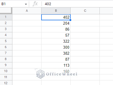
In most cases, this is all one needs to get the job done since a lot can be understood from other aspects of the worksheet, like headers.
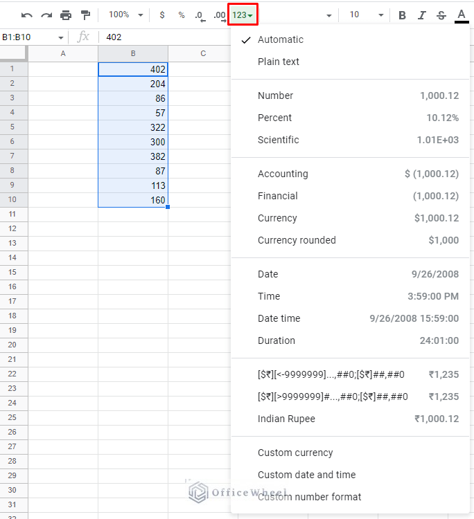
To change the default formatting of a number value, all you have to do is select the number and apply a separate format using either of the following approaches:
Select a new number format from the More formats option:
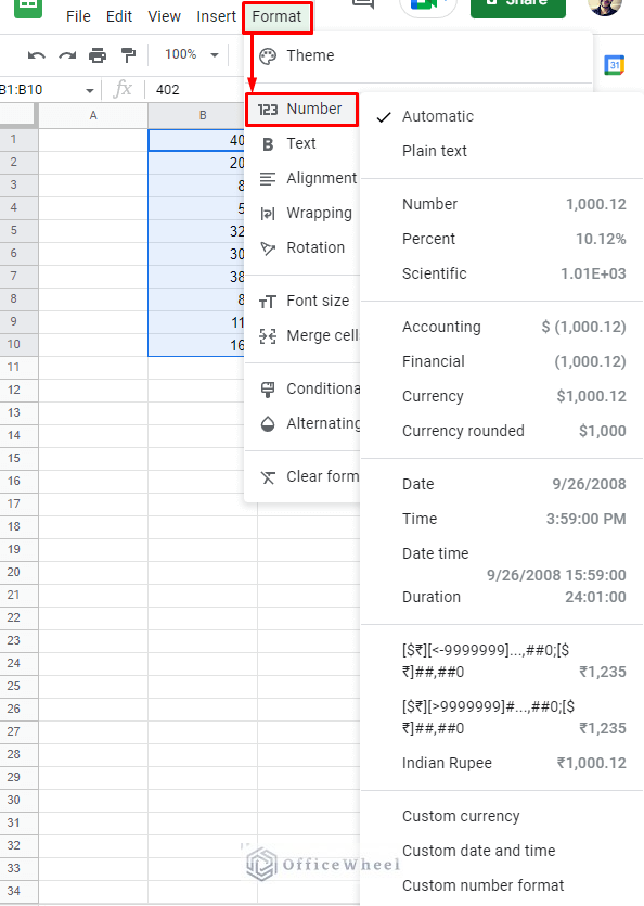
Select a new number format from the Format tab:
Format > Number
For this example, let’s choose the Number format option from the list. The outcome:
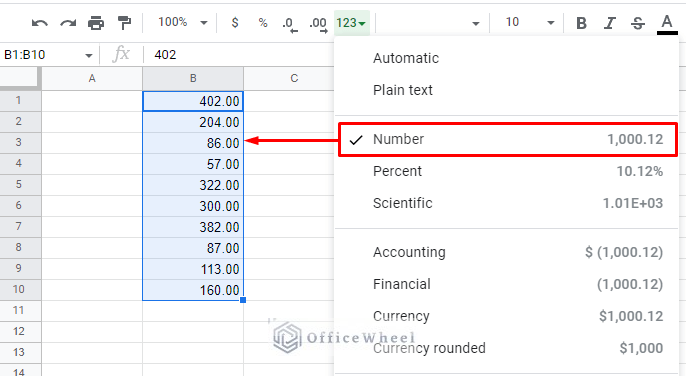
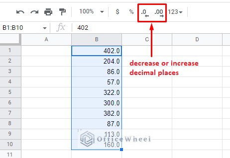
As you can see, this number format comes with decimal places.
To change the number of decimal places of a number in Google Sheets, use the Decrease decimal places or the Increase decimal places options from the toolbar:
This method only applies predetermined number formats in Google Sheets. To further customize numbers, you have to look for other ways, and luckily, Google Sheets provides many.
Change Number Format as Text
Coincidentally, the easiest way to change the format of a number in Google Sheets is to use the TEXT function.
TEXT(number, format)Using this function, we can format any numerical value in any way. For example, to get the same number format that we’ve seen previously (number with 2 decimal places), all we have to do is apply the following formula:
=TEXT(B1,"#.00")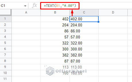
Format Breakdown:
- # (hash): Represents number values where insignificant zeroes (0) are not counted. (e.g. 0.5 will show as .5)
- . (dot): Represents the decimal point.
- 0 (zero): Represents number values where insignificant zeroes (0) will be counted. (e.g. 1.50 will show as 1.50)
Important points to note about the TEXT function:
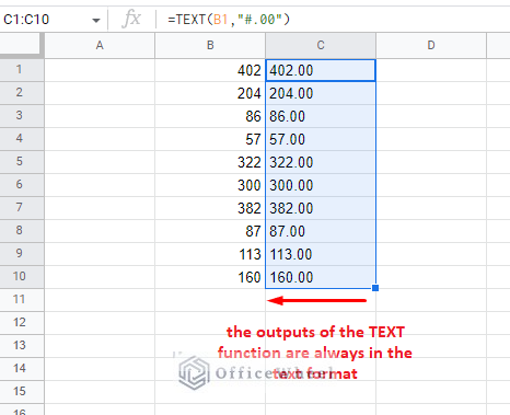
- The function presents the results in a different cell, leaving the source data untouched by any formatting.
- The output is always in the text format.
- You can use the results in any calculation without worry, even if the format is text.
This is obviously not the extent of what the TEXT function can do. You can see more examples of its uses later in the article, like alongside date and currency values.
Learn More: How to Format Numbers as Text in Google Sheets (5 Easy Examples)
How to Change a Date Format in Google Sheets
Dates are one of the more unique number formats of Google Sheets. In certain formats including texts in a date still makes Google Sheets recognize it as a valid number.
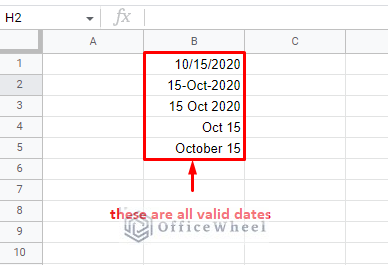
As you can see from the image above, even though the values contain text, they are right-aligned in the cell. This means that these values are numbers in Google Sheets’ eyes, making them valid dates and can be used in calculations.
This also means that we can use the TEXT function to format these dates.
Here is a table with some potential formats that can be applied using TEXT and their results.
| Date Format Code | Result |
|---|---|
| dd-mm-yyyy | 25-2-2022 |
| mm/dd/yyyy | 2/25/2022 |
| MMMM d, YYYY | February 2, 2022 |
| dd-MMM-YYYY | 02-Feb-2022 |
| MMM d, YYYY | Feb 2, 2022 |
| mmm-yy | Feb-22 |
| dd MMM YYYY | 02 Feb 2022 |
| dddd | Wednesday |
| ddd, MMMM DD YYYYY | Wed, February 02 2022 |
Where:
- D or d: Represents date or day.
- M or m: Represents month.
- Y or y: Represents year.
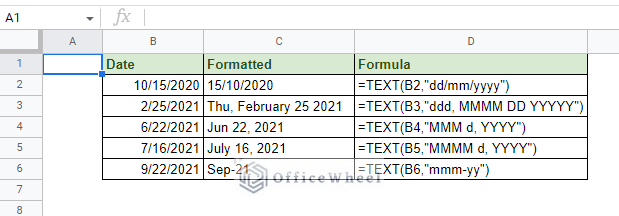
Some examples with some random date formatting in the worksheet with respective formulas:
Learn More: How to Format Date in Google Sheets (3 Easy Ways)
How to Change Currency Format
Currency is just another type of number format that conveys a different meaning. This meaning is primarily carried by the symbol of the currency.
So basically, what we are formatting here is the symbol.
Consider the following dataset:
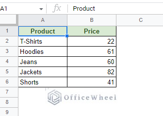
As it stands, we can’t know the actual values of these products. We have a number, yes, but no measure of the magnitude. That will be done by currency.
To format these numbers with the default currency of the application, simply select the cells and click on the Format as currency icon. It is the dollar sign ($) icon in the toolbar.
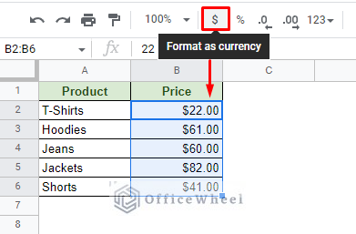
The numbers have been successfully formatted to the USD ($) currency.
The currency formatting does not only change the formatting of the selected numbers, but also that of any results derived from it.
Here is an example of using the recently formatted currency values in a calculation with sales tax:
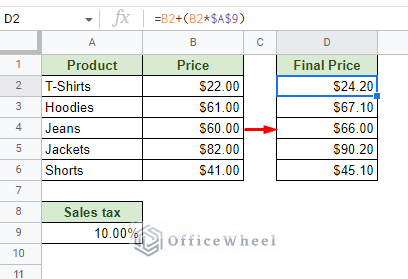
Even though the formula cells weren’t previously formatted, the results appear in the currency format.
The currency format takes precedence in a calculation.
How to Change Currency Type
If the USD is not what you are looking for, then worry not, changing the currency type is also as simple.
Select the cells you want to change the currency symbols of and navigate to the Custom currency option from the More formats menu:
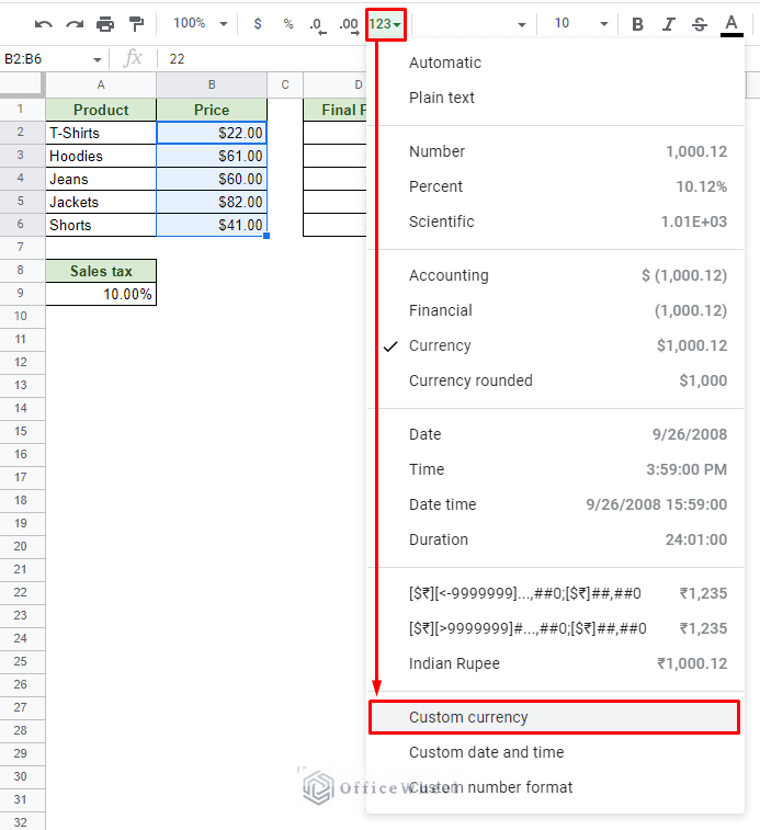
You can also find this option from the Format tab.
Format > Number > Custom currency
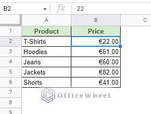
In the Custom currencies window, you’ll find all the available currencies.
You can even search for the currencies that you want and then Apply.
Format Currency as Text
All you have to do is include the currency symbol before the number format in the format field of the TEXT function.
An example formula for changing USD ($) to Pounds (£):
=TEXT(B2,"£#.00")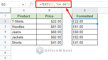
Learn More: How to Format Currency in Google Sheets (An Easy Guide)
Custom Number Formatting in Google Sheets
Google Sheets provides us with a powerful tool to help users format numbers by breaking them down to their basic data values. That is with the Custom Number Format feature.
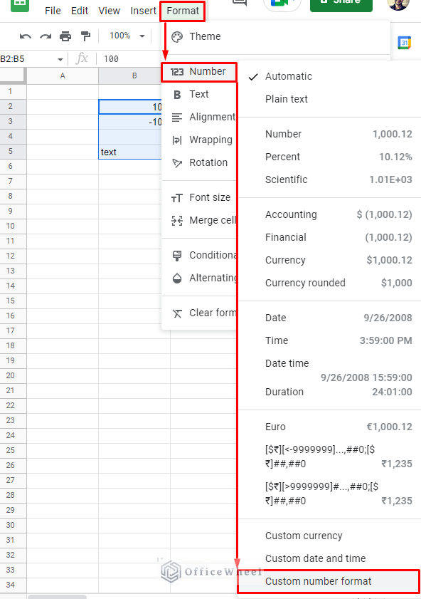
To can access this feature right from the More formats menu or the Format tab of Google Sheets:
Format > Number > Custom number format
Before we get on to the use cases, let’s first understand these “data values” that this feature customizes numbers with.
The Structure of Custom Number Format
The structure of the Custom Number Format can be split into 4 different data values:
- Positive
- Negative
- Zero
- Text
Each of these data is separated by a semicolon (;) in the Custom Number Format window:
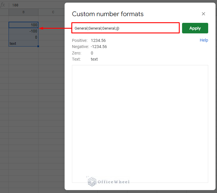
As we can see from the image above, each of these data types corresponds to their named values: positive numbers, negative numbers, zero values, and text.
This means that we can apply different customization in each of these fields to affect the respective values.
Currently, we are just using the “General” keyword as a placeholder to represent no change. In this case, the Text field is unique with the “@”.
Let’s see what happens when we apply the following formatting:
#.00;[Red]General;"zero";"This is Text"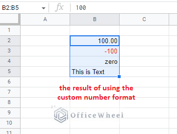
Format Breakdown:
- Positive numbers will have 2 decimal places.
- Negative numbers will have red color characters.
- Zero values will show the text “zero”
- We are replacing any text value with the “This is Text” message.
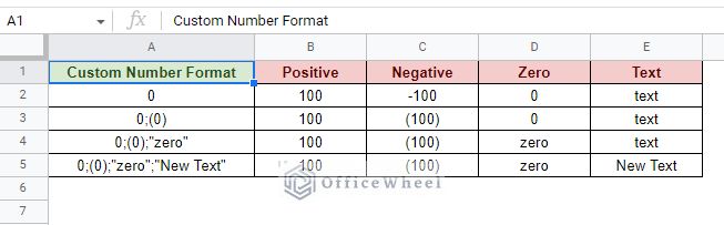
You do not have to use all the rules since the format is read from the left side.
For example, to format negative numbers, we have to first include the formatting of the positive ones. To format zero values, we must first include the formatting of positive and negative values, and so on.
Let’s have a look at a few practical examples.
I. Formatting Phone Numbers using Custom Number Format
For our first example, we will format the following numbers to the phone number format:
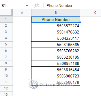
A phone number usually consists of a 3-digit region ID followed by a whitespace and the rest of the digits. The fictional numbers that we have include the 3-digit location ID followed by 7 digits.
The phone number format can also consist of symbols like parentheses around the region ID and a prefix plus (+) symbol.
So, the conversion will be something like this: 5503572274 to +(550) 3572274.
The custom number format is:
+(000) 0000000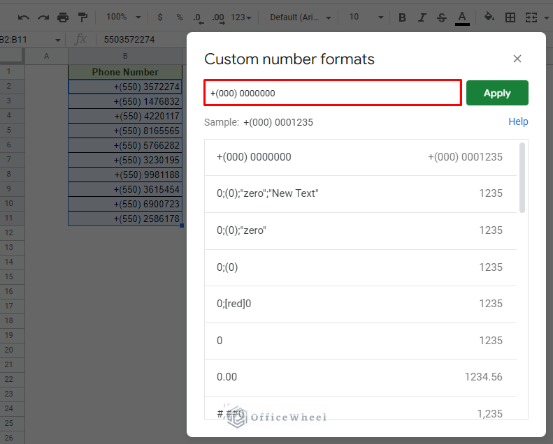
Beyond the symbols and the whitespace, the digits of the phone number must be represented by 0s. Also, the number of 0s must be the same as the digits of the phone number.
II. Change Date Format with Custom Number Format
Previously, in this very same article, we used the text function to format date values in Google Sheets. It had its own advantages but let the results in the text format.
An example of the TEXT formula:
=TEXT(B2,”dd/mm/yyyy”)What this formula does is that it takes a date value and formats it to the dd/mm/yyyy format.
On the other hand, with the Custom Number Format feature, we will take the formatting formula from TEXT’s format field as it will work the same way. Thanks, Google!
On top of that, the formatting will be applied over the existing date, leaving the values as numbers, unlike with the TEXT function.
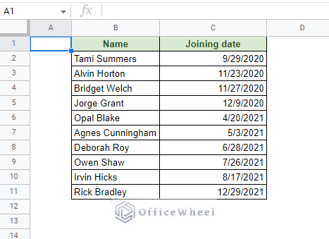
To show this process, we have the following dataset where we want to format the dates to look something like this: Sep-29 (2020).
The custom number format formula is:
mmm-dd (yyyy)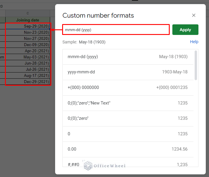
The fundamental date format is the same for both the TEXT function and Custom Number Format.
You can use it in both methods.
Removing Custom Number Formats in Google Sheets
Usually, to remove formatting in Google Sheets you’d use the Clear formatting option from the Format tab (Keyboard Shortcut: CTRL+\).
Format > Clear formatting
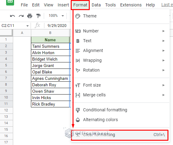
However, Custom Number Formats cannot be removed by the Clear formatting feature.
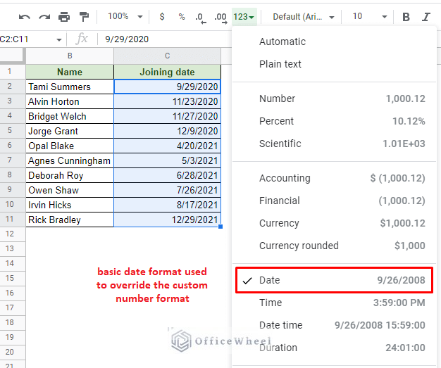
The only way to remove custom number formats in Google Sheets is to override the existing format with a basic format or another custom format.
Change a Number Format from the Google Sheets Mobile App (Android/iOS)
The Google Sheets Mobile application is quite seamless whether you are using it from an Android or an Apple device.
It also has almost all basic and a few advanced features that we can use in the browser version.
While we can format numbers quite well in the mobile app, it does not have the Custom Number Format feature. However, it has more than enough to satisfy most needs.
For this example, we will try to change the date number format using the Google Sheets mobile app.
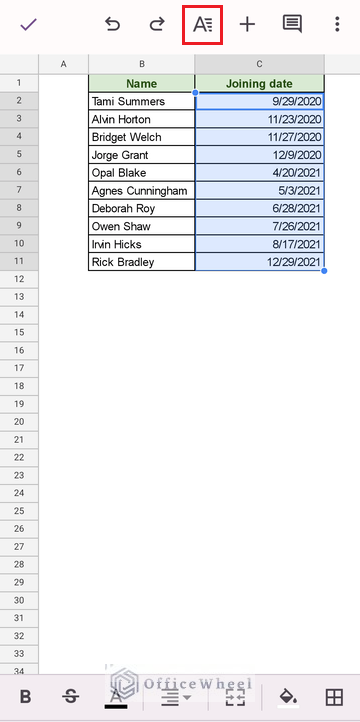
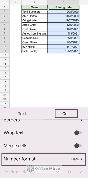
Step 1: Select the cells that contain the date values. Tap once on the first cell to select it. Tap again and drag to select the rest of the cells.
Once selected, click on the Format icon (see image).
Step 2: Move to the Cell tab. Here, select the Number format option.
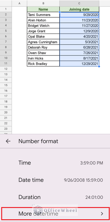
Step 3: Scroll down to the bottom to find the More date/time option and select it. This is the closest we can get to applying a custom date format.
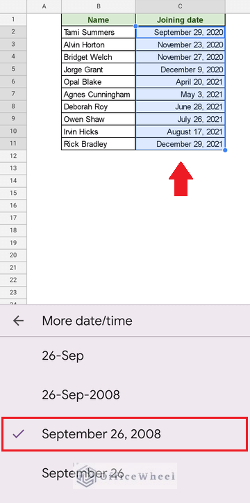
Step 4: Select the date option that suits your requirements and see the results.
Final Words
With that, we conclude our simple guide on how to change a number format in Google Sheets.
Know that all we have done is only touch on the fundamental processes of number formatting available to us in Google Sheets. With time and experience using these features and techniques, you will see that there are a whole lot more available customizations to utilize yet.
Feel free to leave any queries or advice you might have in the comments section below.