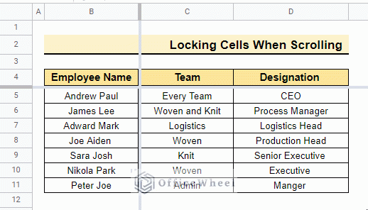
Working on a large dataset is very normal in our day-to-day work life. But sometimes you need to find out very old values and to find the old values we need to scroll down in google sheets. Well, the difficulties start from here. Because once you scroll down and reached the required data the header row is already gone and now you don’t know which data stands for what. But in your google sheets, you can lock cells to get quick search results. In this article, we will learn how to lock cells in google sheets when scrolling.
Here is the overview of this article. You will learn more once you go through the total article.
A Sample of Practice Spreadsheet
You may copy the spreadsheet below and practice by yourself.
2 Ways to Lock Cells in Google Sheets When Scrolling
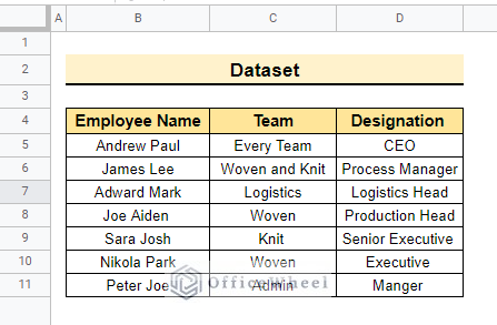
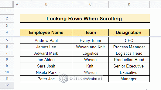
The below dataset contains Employee Name, Team, and Designation. This dataset represents the employees with their team and their designation. It is like an induction chart. Now we will lock some specific row or column so that when the dataset extends the header row and the names of the employees are visible.
1. Locking Row Cells
Therefore, we will lock the header rows in google sheets when scrolling. Imagine this company is new and keeping track of these employees. Now the number of employees are increasing and the team and designation as well. So, it is a matter of time before this induction chart will be very large and difficult to operate. In that case, if we lock the header row then keeping track of the data will be much easier. Follow the steps below to execute this process.
📌 Steps:
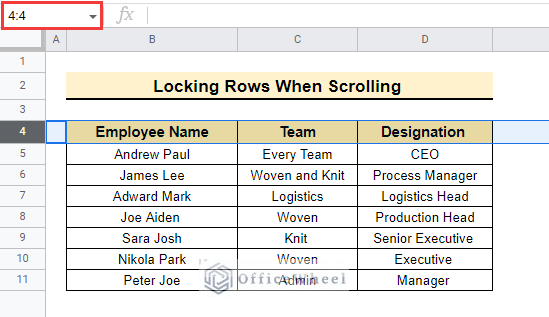
- First, put the cursor on the left side of the header row and click on the header row number as below. Here the header row is number 4.
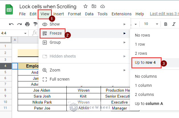
- Then, select View >> Freeze >> Up to row 4 to freeze the top 4 rows as the header row is the 4th row.
- In the end, the final output is as below.
Read More: How To Lock Rows In Google Sheets (2 Easy Ways)
2. Locking Column Cells
Here, we will lock the column cells in google sheets when scrolling. In case we add any project, office time, and other necessary information to this induction chart then the name of the employee should be visible every time. So, follow the steps to lock the cells.
📌 Steps:
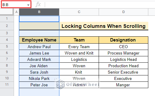
- Initially, select the total column B by clicking on column name B as below.
- As we need to lock the employee names so we will lock till column B.
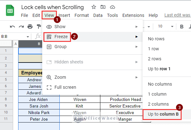
- Afterward, select View >> Freeze >> Up to column B and lock the sheet till column B.
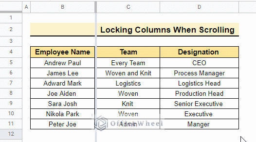
- Consequently, the employees’ names will be always visible in the dataset.
- Finally, the output of this process is below.
- You can also lock more than one row in this dataset. Suppose you want to lock Team also then you need to select column C and lock up to column C.
Read More: How to Lock a Column in Google Sheets (Simple Examples)
Things to Remember
- You cannot lock any merged column. If the column is merged then first you need to unmerge the cells.
- You cannot merge locked cells and unlock cells together. If you want to merge cells together first make sure both are unlocked.
Conclusion
In this article, we explained how to lock cells in google sheets when scrolling. Hopefully, these procedures will help you apply this method to your dataset. Please let us know in the comment section if you have any further queries or suggestions. You may also visit our OfficeWheel blog to explore more Google Sheets-related articles.
Related Articles
- How to Protect Formulas in Google Sheets (2 Quick Ways)
- Lock Cells with Formula in Google Sheets (with Easy Steps)
- How to Lock Certain Cells in Google Sheets (With Quick Steps)
- Protect Range in Google Sheets (Easy Examples)
- Conditional Locking Of Cells In Google Sheets (Easy Steps)
- Protect Sheet From View in a Google Spreadsheet (2 Ways)

