In professional work, we are often asked to tackle worksheets that have large amounts of data. In such cases, it is imperative that we freeze up our table headers to keep track of any data entry that might occur in the lower rows of our worksheet.
So, in this article, we will be looking at multiple processes of how to freeze rows in Google Sheets, as well as undo any changes.
But first…
Why do we need to freeze rows?
When handling a long list of data, it can be crucial to lock the column headings so that as you scroll down your worksheet, you are aware of the kind of column you are working with.
Scrolling down a regular worksheet:
Scrolling down a worksheet with a locked/frozen header row:
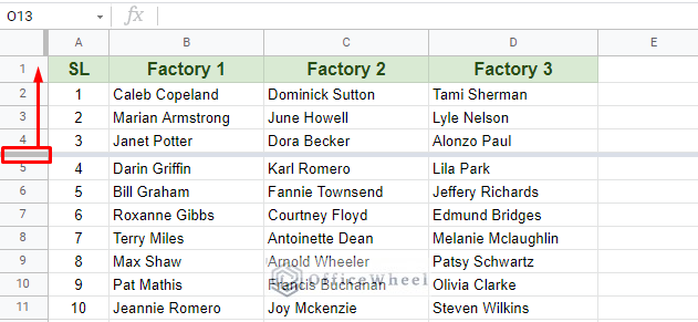
As you can see, even if we scroll down the rows, our headers are always visible, making it easy for us to input data (names) into the correct columns.
This is one simple example of how freezing rows can be useful for your spreadsheet.
Now, let’s look at a few ways of how we have been able to achieve it.
3 Ways to Freeze Rows in Google Sheets
1. Freeze Rows in Google Sheets Using Mouse (Dragging the Row Pane)
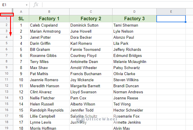
The simplest way to freeze rows in Google Sheets is by dragging and dropping the Row pane (the horizontal pane at the top-left corner of the sheet).
This locking of rows is not limited to row number 1 only. You can drag the Row pane to any row as needed to freeze.
In other words, you can freeze multiple rows in this way.
Note: To select the Row pane, make sure your mouse cursor is in the hand cursor form (see the image above). Dragging with any other cursor might mess up your worksheet. In such cases, you always Undo (shortcut: CTRL+Z).
2. Freeze Rows in Google Sheets Using the View Tab
The classic way to freeze panes in spreadsheets, be it Excel or Google Sheets, has always been to do so from the Toolbar menu. Namely the View tab.
The keyboard shortcut to access the View tab:
- PC: ALT+V (Chrome) or ALT+SHIFT+V (other browsers)
- Mac: CTRL+OPTION+V
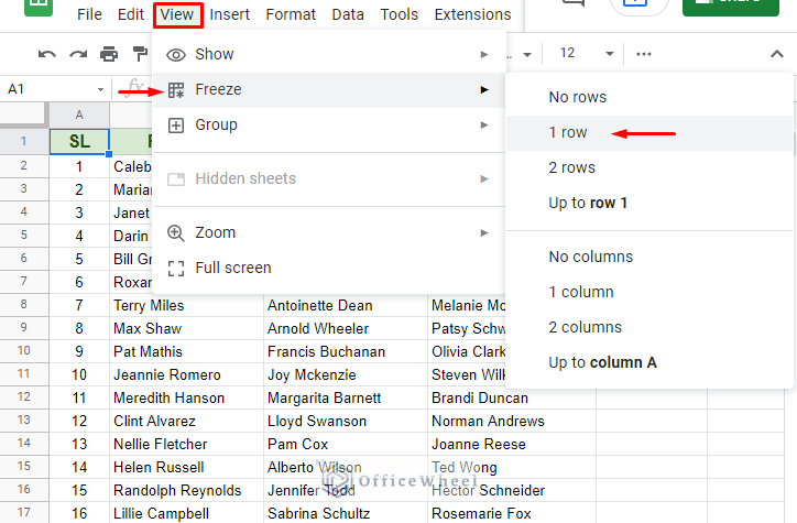
From here, navigate to Freeze and select the 1 row option to freeze the first row.
View tab > Freeze > 1 row
You can select the 2 rows option to freeze the first two rows.
Freeze Multiple Rows With Toolbar
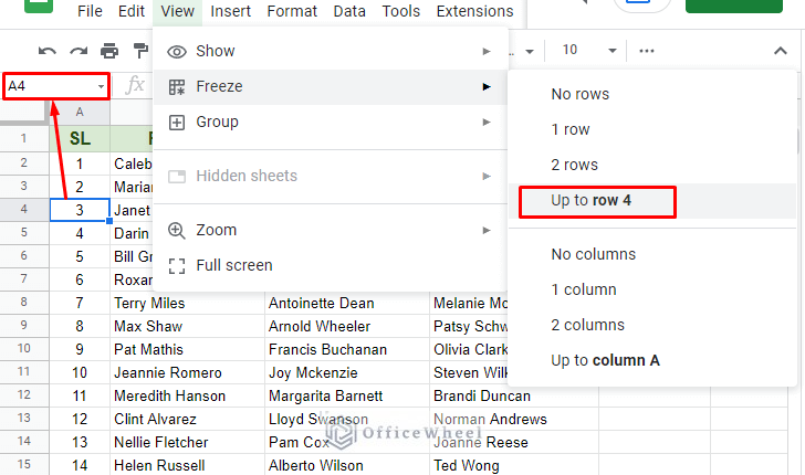
To freeze multiple rows, make sure to keep your active cell on the row until which you want to freeze.
In this instance, we have kept our active cell as A4. Thus, you can see that in our Freeze rows option we have Up to row 4 option available.
Our result:
Read More: How to Freeze 3 Rows in Google Sheets (2 Quick Ways)
3. Freeze Rows in Google Sheets Mobile App
Freezing rows in Google Sheets’ mobile application is equally simple. That goes for both Android and Apple devices.
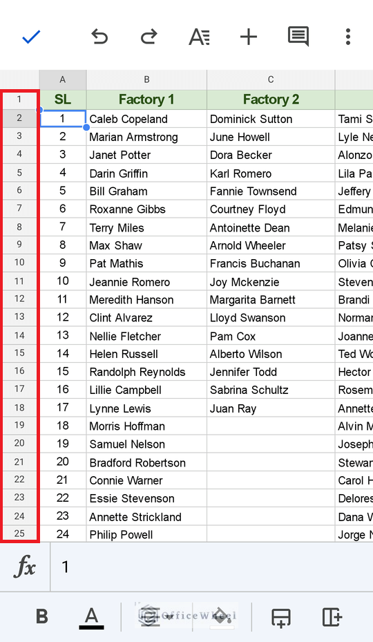
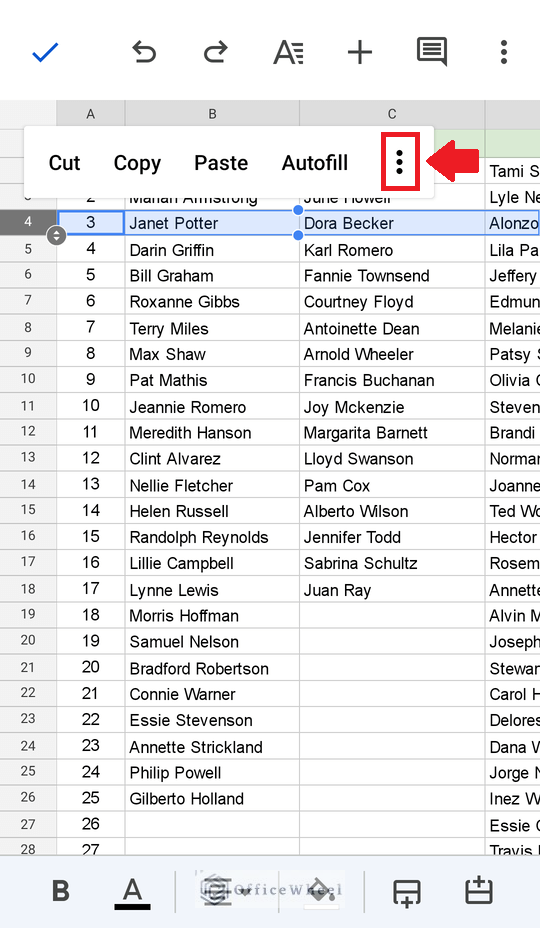
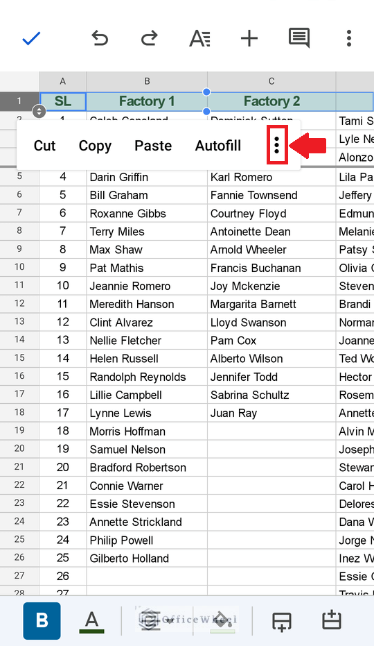
Step 1: Tap and hold the row header where you want to place your freeze. The row headers are highlighted in the image below.
Step 2: An option tray will pop up. Expand the options by tapping the vertical 3-dot icon to the right.
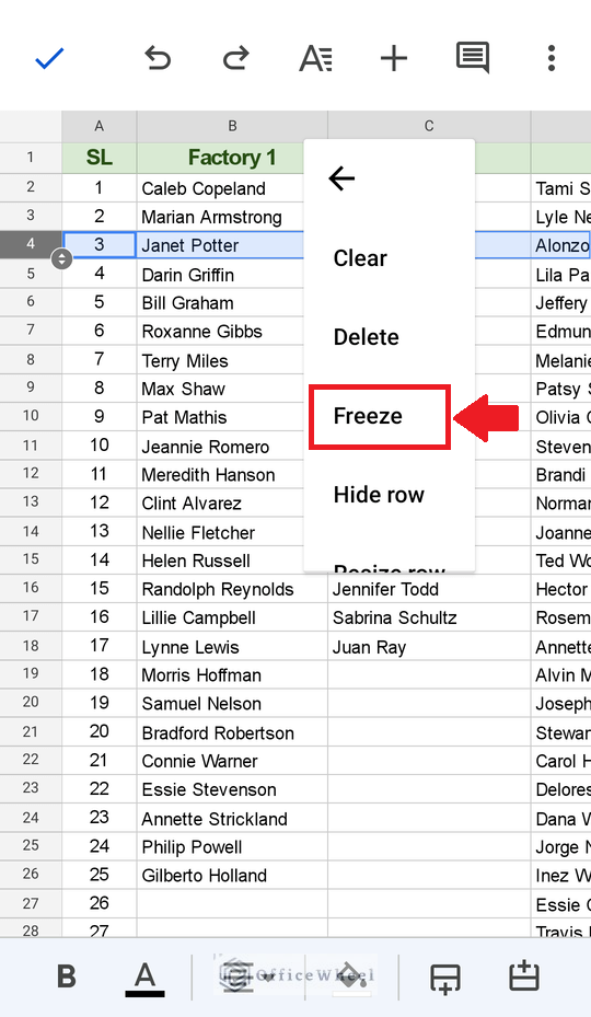
Step 3: Tap on the Freeze option.
With that, we have discussed all of the ways by which you can freeze rows in Google Sheets.
But it is also important to know how to reverse the processes that you have just learned, that is to unfreeze rows in Google Sheets.
We will look at that in the next section.
How to Unfreeze Rows in Google Sheets
1. Unfreeze Rows on Your Browser
The first way is as simple as dragging the Row pane.
Simply select the row pane, click and drag it upward until it is back in its default position.
Note: Make sure to click and drag only when the hand cursor appears.
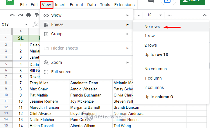
The next way is to use the View tab.
Navigate to the View tab up top and select the Freeze option. Here select the No rows option to remove all frozen rows in your worksheet.
2. Unfreeze Rows on Your Mobile Device
Unfreezing rows in Google Sheets from a mobile device follows a similar process as freezing.
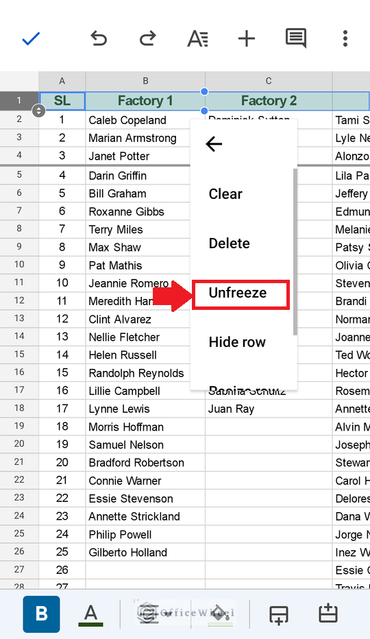
Here, just tap and hold the first-row header, row 1, until an option tray appears. Tap on the vertical 3-dot icon to expand the options available.
Here, tap on the Unfreeze option.
Final Words
Freezing rows and columns in Google Sheets is a fairly easy affair, as long as you know what to look for.
We hope that this article has helped you understand the different approaches to freeze rows, for both your computer and mobile device. However, if you are looking for ways to protect and lock rows, then please follow our How To Lock Rows In Google Sheets article.
Please feel free to leave any queries or advice you might have for us in the comments section below.