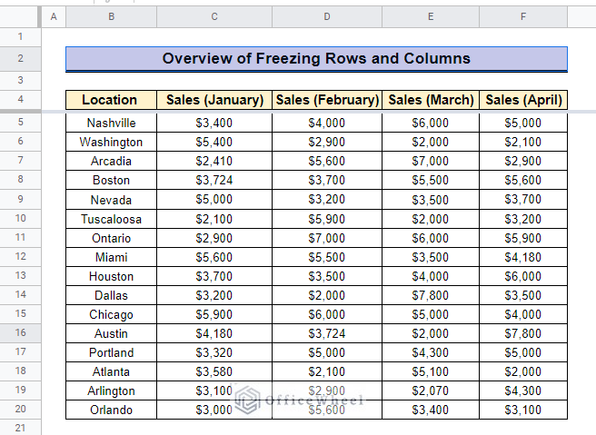
In Google Sheets to handle a large amount of data, freezing rows and columns is a very useful feature. By freezing important rows and columns you can easily manage thousands of data. In this article, we will explain how to freeze rows and columns in Google Sheets.
A Sample of Practice Spreadsheet
You can download Google Sheets from here and practice very quickly.
Why Do We Need to Freeze Rows and/or Columns in Google Sheets?
When dealing with a huge dataset, the freeze feature can freeze specific rows or columns in your spreadsheet in Google Sheets so that you can keep viewing them as you browse through your dataset. There are some basic causes why we generally need to freeze rows or columns:
- For large datasets, we need to freeze the headers to input data in a proper way.
- When you want to compare data with other data you have to keep the columns or rows locked in the entire spreadsheet.
- To mark some special data which is important for the entire spreadsheet, you can freeze them and can see them when browsing the entire spreadsheet.
2 Simple Approaches to Freeze Rows and Columns in Google Sheets
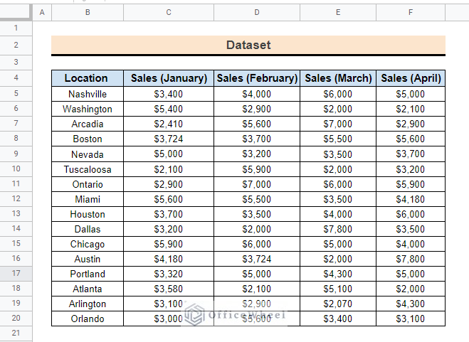
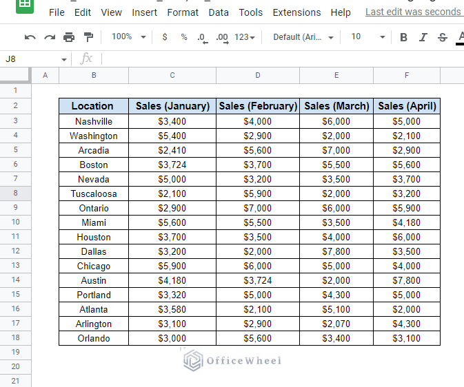
You can freeze the rows and columns by applying the two simplest techniques. To show these approaches we develop a dataset that mainly shows the monthly sales of different locations.
1. Click and Drag Freeze Panes
The easiest way to freeze columns and rows is to click and drag the freeze panes. To do so,
Steps:
- First, go to the top left corner of the spreadsheet. You will find gray panes situated both horizontally and vertically.
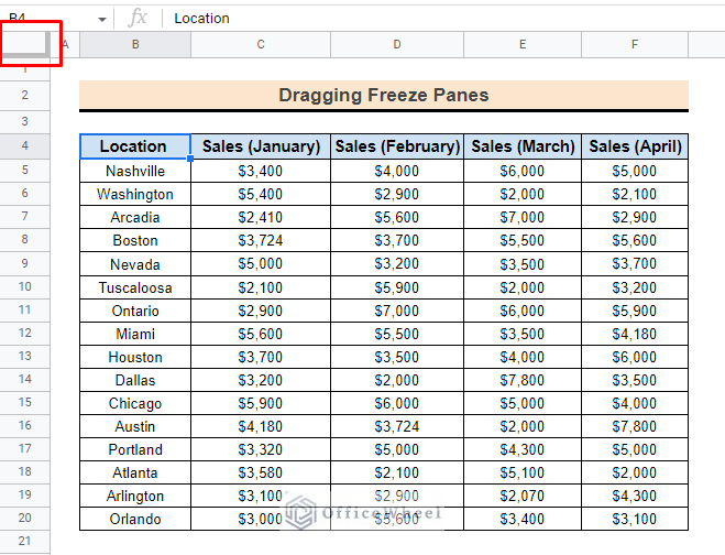
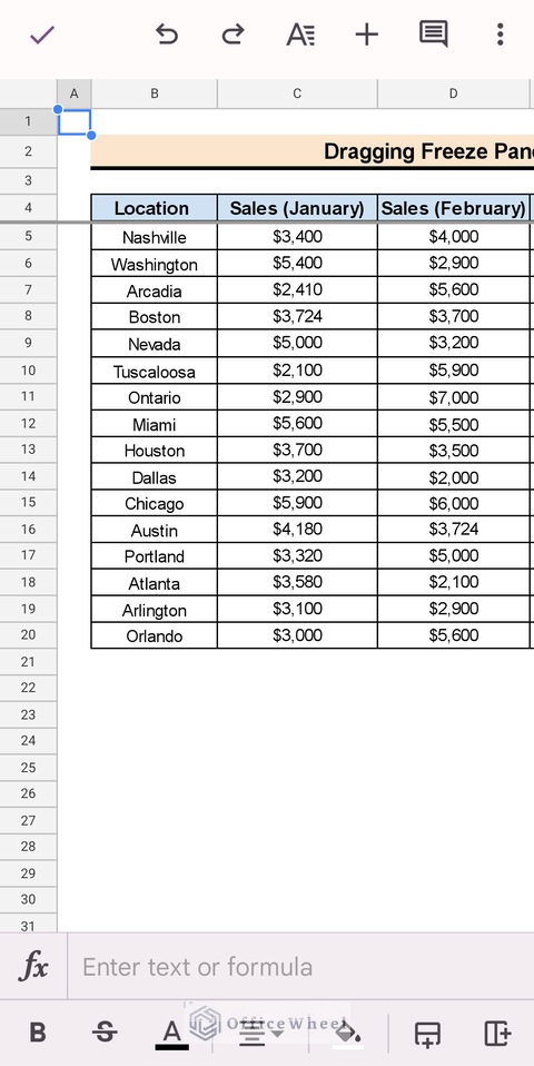
- When taking the mouse over the gray panes it turns into a hand icon. Then you can drag the gray pane horizontally or vertically. Here, we drag down the frozen handle from row 4.
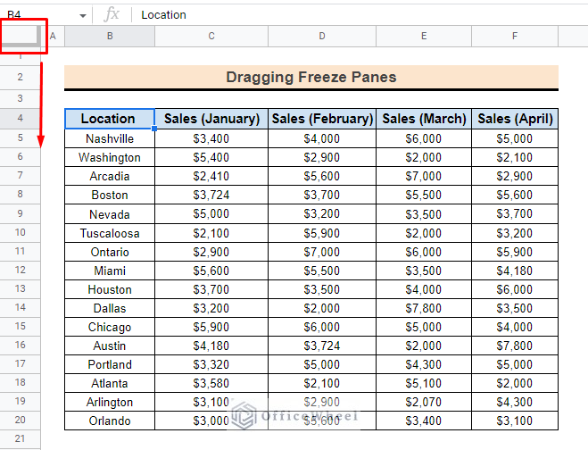
- You can see the whole process at a glance.
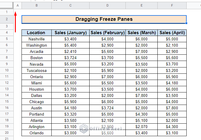
- You can also apply the same procedure to drag the vertical freezing pane.
3. Utilize View Menu
You can also use the View menu from the feature bar to freeze columns and rows in the spreadsheet. To apply the method,
Steps:
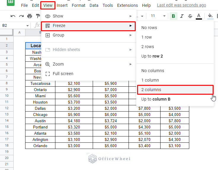
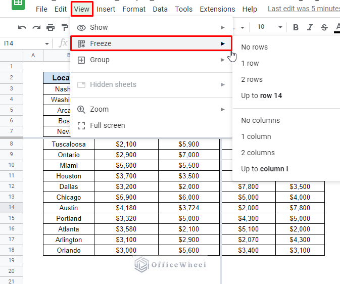
- First, go to the View feature and select the Freeze option. Here, you will find multiple freezing options for your rows as well as columns.
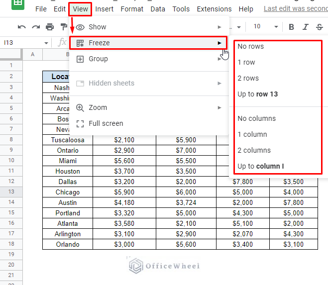
- You can select any number of columns and rows you want to freeze. Here we select 2 rows to freeze.
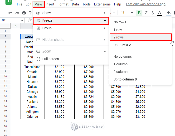
- Then choose 2 columns to freeze.
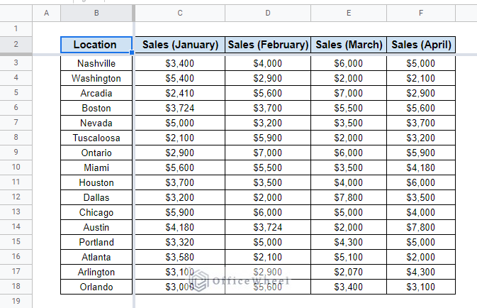
- After selecting freezing columns and rows the spreadsheet looks this way.
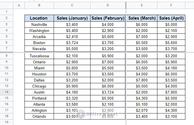
- When you browse the spreadsheet, the first 2 columns and rows remain frozen.
- You can apply the same procedure for multiple columns and rows also.
(Android/iOS) How to Freeze Rows and Columns in Google Sheets from Mobile Device
You can also freeze both columns and rows in Google Sheets displayed on your android or iPhone. To do so in the beginning you have to open a spreadsheet in the Google Sheets App.
Steps:
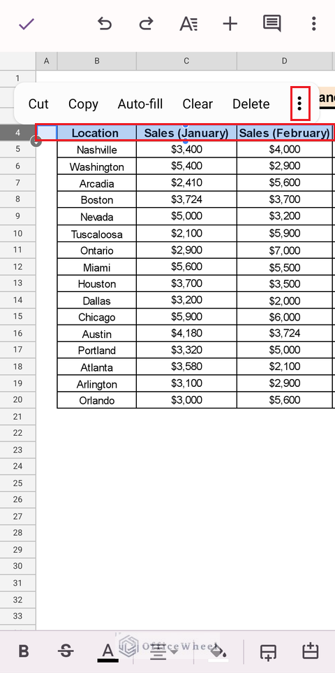
- Click on the rows or columns and you will find options. Select the three-dot icon to open more options.
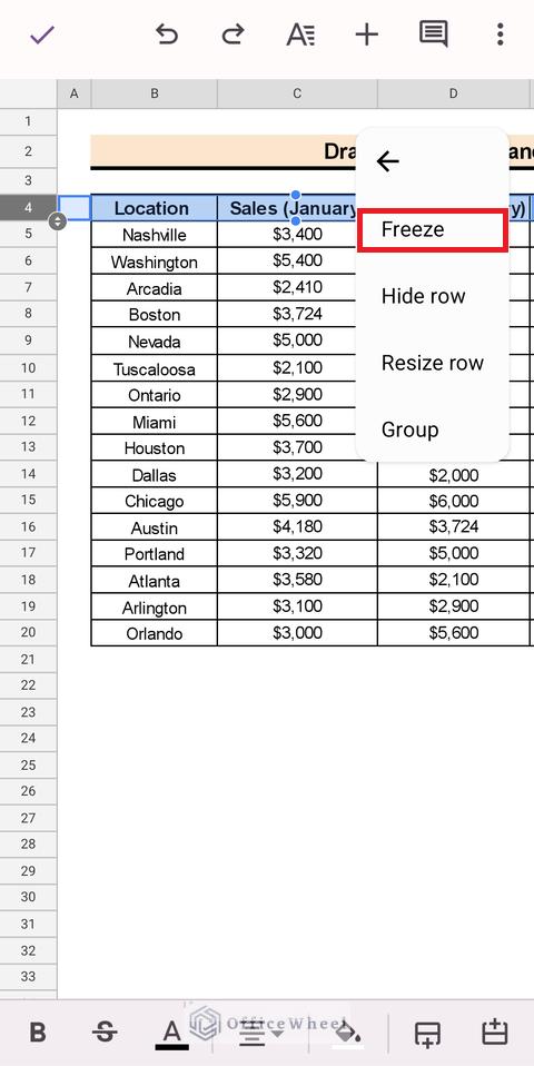
- Then from more options choose the Freeze option.
- Finally, you will find the selected rows or columns are frozen.
Read More: How to Freeze Specific Columns in Google Sheets (3 Quick Ways)
How to Unfreeze Rows and Columns in Google Sheets
Unfreezing rows/columns is quite simple and quick to execute in Google Sheets. You have to apply the reverse technique of the following two methods for unfreezing respective rows and columns.
1. Unfreeze by Dragging Freeze Panes
Once you freeze any row or column, you find the gray color pane on that column or row. Then, just drag the pane and keep it back to the top left corner of the spreadsheet.
2. Unfreeze by View Menu
To unfreeze from the View menu.
Steps:
- First, go to the View bar and select the Freeze option.
- After that select the No columns or No rows option for making the freeze rows and columns unlock.

- Finally, you will find all frozen rows or columns are unfrozen.
Things to Remember
- You cannot freeze columns or rows from the middle of the spreadsheet.
- You cannot freeze columns or rows in one go. You have to freeze them one after one.
Conclusion
In this article, we explained how to freeze rows and columns in google sheets. We believe you can apply the methods in your dataset. If you have any queries or suggestions, please let us know in the comment section. You may also enhance your expertise in Google Sheets by visiting the OfficeWheel website.