How to Freeze Panes in Google Sheets (3 Simple Ways)

If you have a large dataset with many rows and columns, it can be difficult to understand if some of the rows and columns are not visible. Freezing panes in Google Sheets is a useful feature that allows you to lock certain rows or columns in place while scrolling through the rest of the sheet. This can be especially helpful when working with large datasets or tables that have a lot of columns or rows. In this article, we will discuss the ways to freeze panes in Google Sheets.

The above image is an overview of the article to freeze panes in Google Sheets. In this article, we will learn the ways to freeze panes in Google Sheets.

3 Simple Ways to Freeze Panes in Google Sheets

Freezing panes in Google Sheets is a useful feature that can help you navigate large datasets or tables more easily. There are several different methods for freezing panes, including using the View menu, the right-click menu, etc.

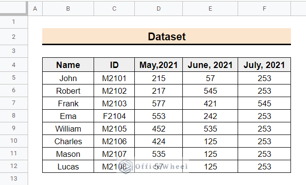
Suppose you have a dataset of monthly unit sales of the employees of a company. Now you need to freeze column B as well as row 4. Follow the below methods to freeze columns and rows in Google Sheets.

1. Using the Mouse Click and Drag

Using the mouse click and drag is the easiest and quickest method to freeze pans in Google Sheets. Follow the below steps to use the mouse click and drag to freeze rows and columns.

📌 Steps:

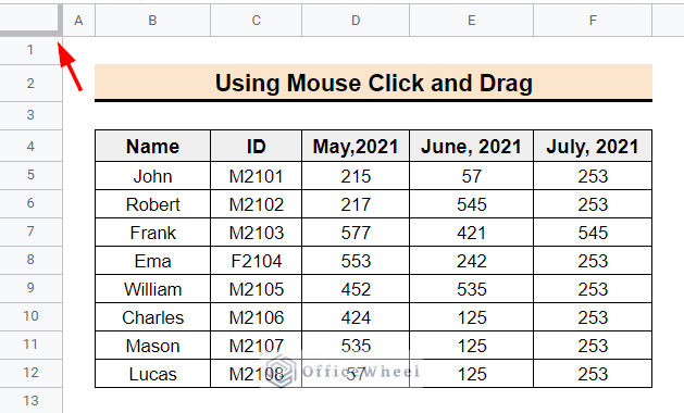
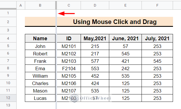
• First, go to the top left corner of the sheet and find the blank grey box with two thick gray lines.

• Now, if you hover the cursor over the lines a hand icon will appear. To freeze column B, click the vertical line using the hand icon and drag the line to the right-hand side border of column B.

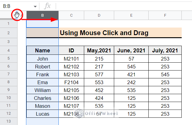
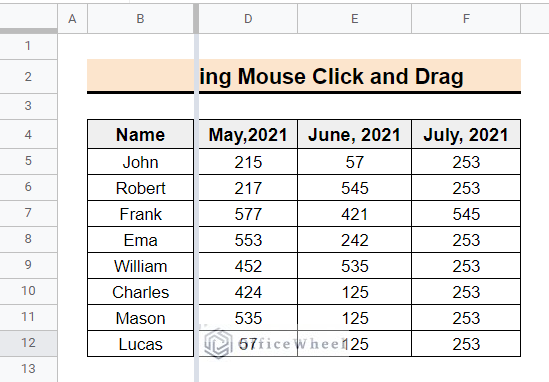
• Finally, the thick vertical line will locate on the right side border of column B and columns up to column B will freeze.

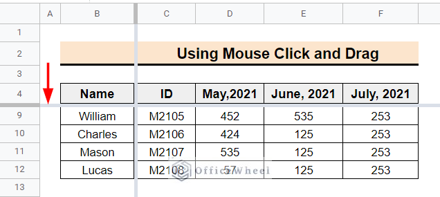
• After that, you will see column B remaining freeze while you scroll to the right side of the dataset.

• Similarly to freeze row 4, click and drag the horizontal line of the blank grey box to the bottom line of row 4.

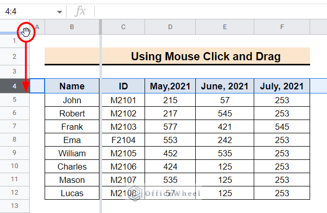
• As a result, the row up to row 4 will freeze, and when you scroll down, rows up to row 4 will remain still.

2. Applying Freeze Option of Google Sheets

You can use the option Freeze from the top menu to freeze panes in Google Sheets. Here are the steps to freeze panes in Google Sheets by applying the option Freeze.

📌 Steps:

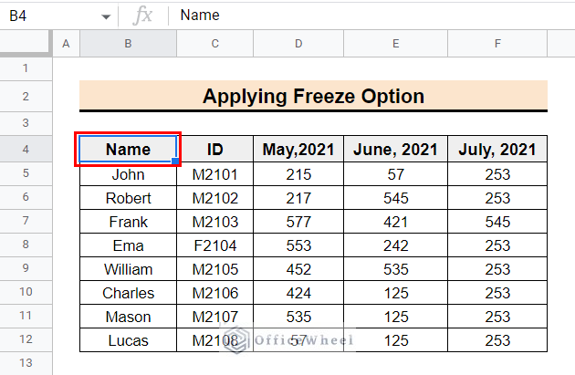
• In the beginning, select cell B4 to freeze column B and row 4.

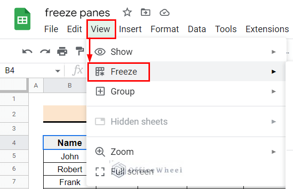
• Now from the top menu select options View >> Freeze.

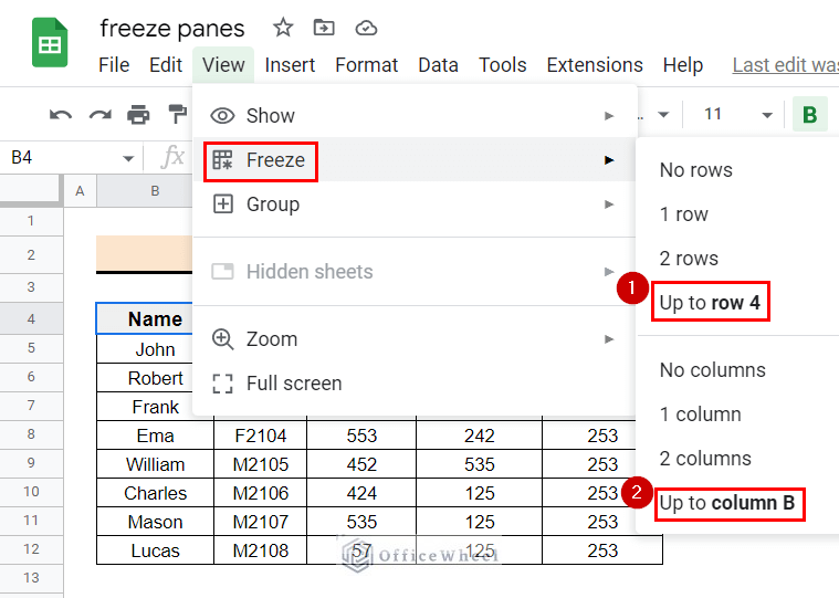
• Following that, choose Up to row 4 option from the Freeze options to freeze the rows up to that point.
• Subsequently, choose Up to column B option in the same way to freeze columns up to that column.

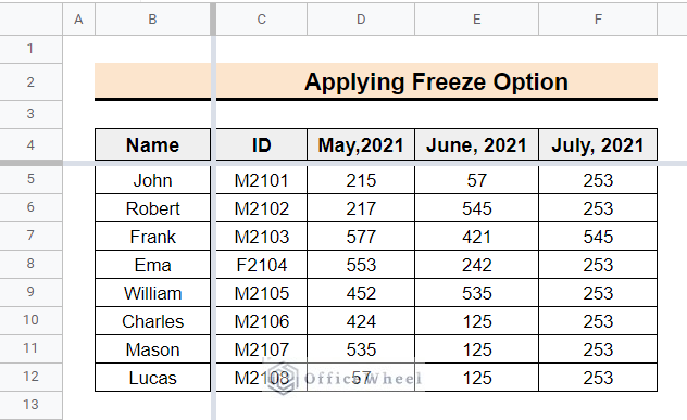
• In the end, you can see the output similar to the following image.

3. Using Right-Click Menu

Accordingly, you can use the context menu from the right-click of the cell up to which you want to freeze panes. Follow the below steps to freeze column B and row 4.

📌 Steps:

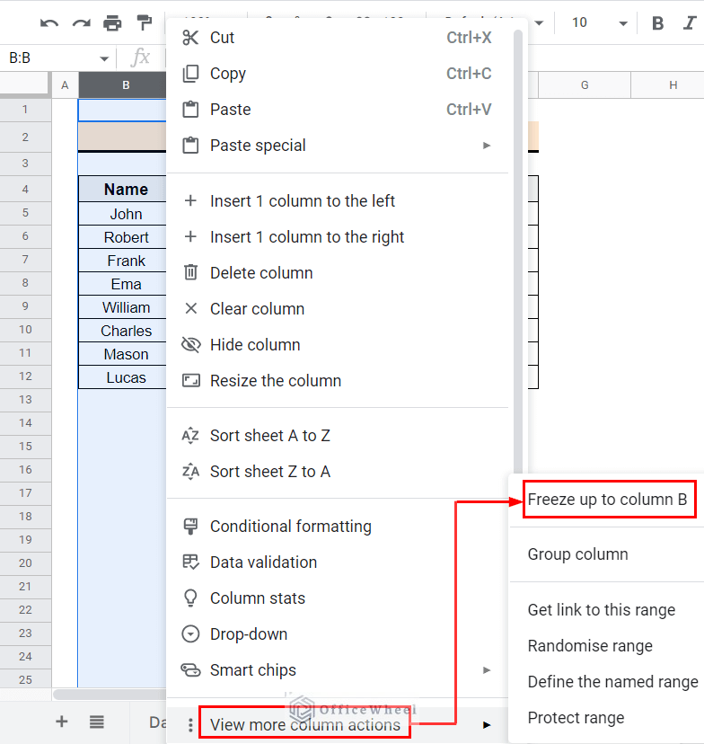
• First of all, select the column or row that you want to freeze. For our case select column B.

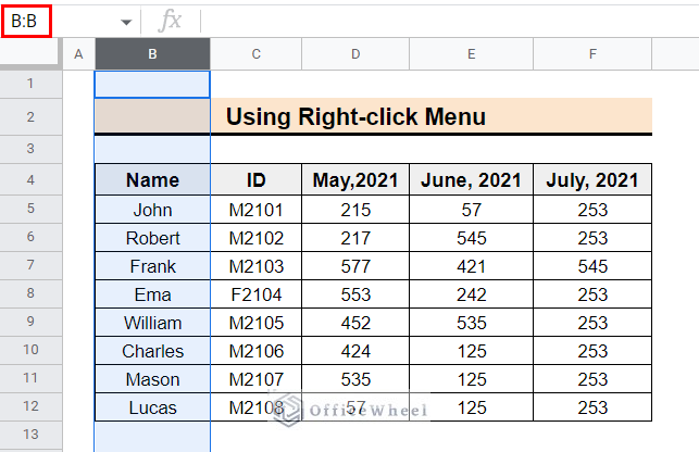
• After that, right-click on column B and from the context menu, select the options View more column actions >> Freeze up to column B.

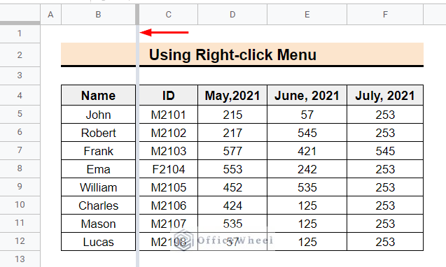
• Now the output will look like the following image.

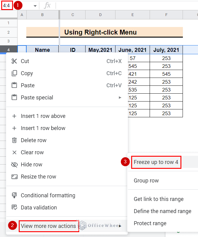
• In the same way, you can freeze row 4 by selecting the options View more row actions >> Freeze up to row 4.

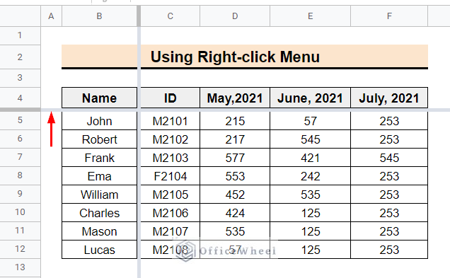
• Lastly, the final output will look like the following image.

Read More: How to Freeze 3 Rows in Google Sheets (2 Quick Ways)

How to Unfreeze Panes in Google Sheets

In a similar procedure to freeze panes, you can also unfreeze the pans in Google Sheets. The easiest way is to use the mouse click and drag method. Follow the below steps.

📌 Steps:

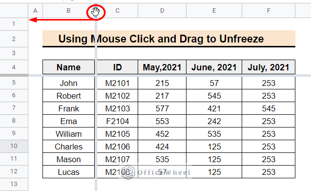
• First of all, hover the cursor over the thick border located at the right-side border of column B. A hand icon will appear. Use the hand tool and drag the thick grey border line to the left-most empty cell.

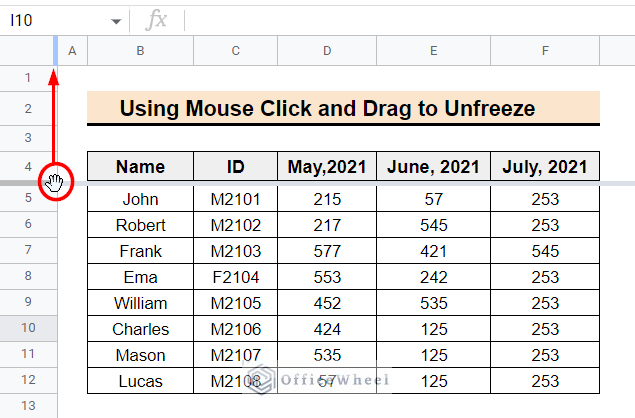
• Similarly, drag the thick grey border line from the bottom border of row 4 to the bottom border of the top-most empty cell.

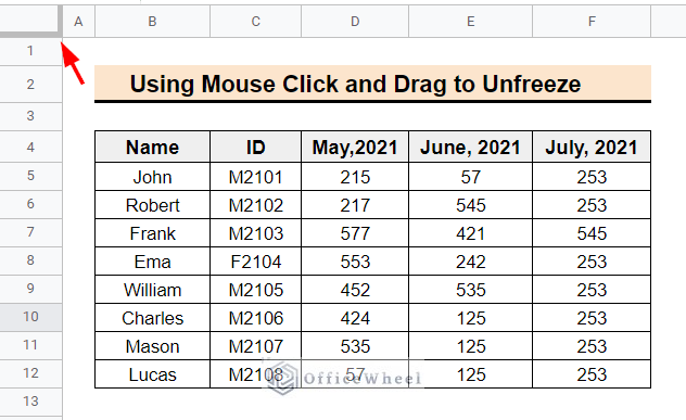
• Lastly, the final output will look like the following image.

Things to Remember

You can freeze columns or rows that are merged with the adjacent columns or rows.

Conclusion

In conclusion, freezing panes in Google Sheets is a useful feature that can help you navigate large datasets or tables more easily. Following the methods above you can quickly freeze panes in Google Sheets. Comment below with your queries and suggestion. Visit the OfficeWheel website to get more Google Spreadsheet-related articles.