Suppose you are working on a dataset where you need to input data every day and the dataset is getting larger every day. In this case, it is a matter of time that if you scroll down the dataset then the header row will be lost. Once the dataset is larger, it will be difficult to operate and very time-consuming as well. But if you freeze your rows then the rows will be locked and if you scroll down the data will remain there. In this article, we will learn how to freeze 3 rows in google sheets.
Here is the overview of this article, you will learn better once you go through the total article.
A Sample of Practice Spreadsheet
You may copy the spreadsheet below and practice by yourself.
2 Simple Ways to Freeze 3 Rows in Google Sheets
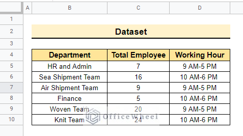
The below dataset contains Department, Total Employee, and Working Hour. That means this dataset represents the total employees of every department and their working hours This table is a schedule table. If you want to meet anyone then you can go through this table and you know the working hour of that employee.
1. Using Menu Bar
Now, we will freeze 3 rows so that the top row always remains visible after scrolling using the following dataset that represents the working hour of different teams in a company. Say, we need to freeze the top so that it always stays at that place and the dataset is easy to operate.
📌 Steps:
- First, select three rows from the dataset. Put the cursor at the very top left side of the dataset.
- Then click on the cell number as the third cell number is three. So select 3.
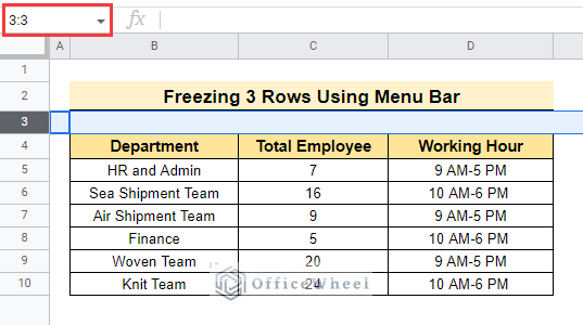
- Select the row number then google sheets will select the entire row as shown before.
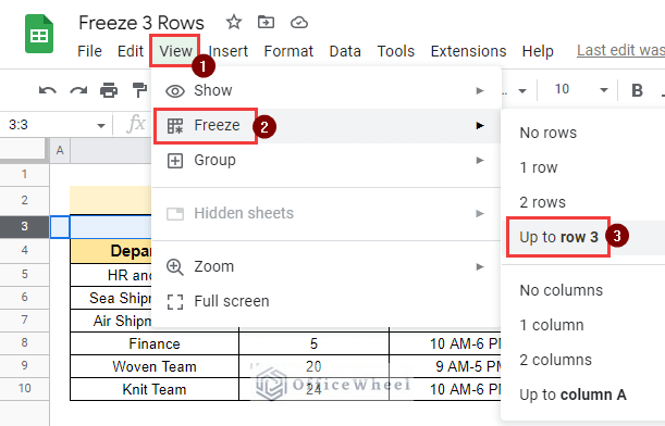
- Afterward, select View >> Freeze >> Up to row 3 to freeze the rows till 3.
- we can also execute this same process using the keyboard shortcut. As this process is convenient and time-saving at the same time.
- To do this, press ALT + V, and the View pane will pop up.
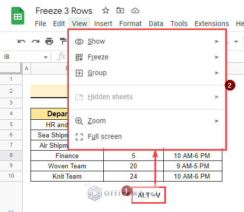
- Now the View pane will pop up now select freeze as shown before.
- Finally, the data is frozen and the final output is below.
2. Dragging Mouse
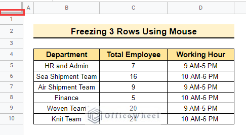
We can also use the mouse to execute freeze rows. This simple way will save you time. This process is quite simple. There is a Row Pane in every google sheet. The row pane is a line in the most top left side shown in the picture.
📌 Steps:
- Select the Row Pane and drag it down to the 3rd row as below to freeze 3 rows.
- Lastly, the final output is below.
Read More: How to Freeze Panes in Google Sheets (3 Simple Ways)
Things to Remember
- If you merge the rows already then you cannot freeze just one row. First, you have to unmerge the row then you can freeze the row.
- Also, you can not lock merged and unmerged cells together. You need to unmerge the cells if you want to lock the cell.
Conclusion
In this article, we explained how to freeze 3 rows in google sheets step by step. Hopefully, this procedure will help you apply this method to your dataset. Please let us know in the comment section if you have any further queries or suggestions. You may also visit our OfficeWheel blog to explore more Google Sheets-related articles.