Google Sheets: Sum of Cells with Text (4 Examples)

In this simple tutorial, we will look at a few example scenarios where we sum cells with text or those that depend on text in Google Sheets.

Note that these scenarios are niche cases and most likely won’t appear in most spreadsheets.

But in case it does appear, it is always better to understand how data is manipulated in the application.

Let’s get started.

4 Examples to Find the Sum of Cells With or According to Text in Google Sheets

1. Sum All Cells Containing Text in Google Sheets

The following worksheet contains a bunch of data: texts, numbers, and even blank cells. We have even sneaked in a number formatted as text.

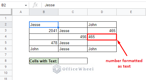
The idea is to count only the cells that contain text values.

Using the COUNTA function to count non-empty cells here won’t work since we have different types of values.

So, we have to perform a count with a condition, and the best way to do that is by using the COUNTIF function.

The formula with the COUNTIF function to find the sum of all text cells in the range is:

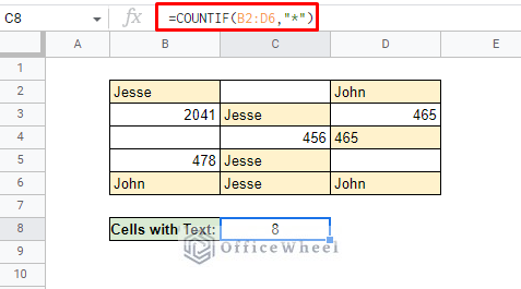
Simple, isn’t it?

The asterisk (*) symbol as a condition makes the COUNTIF function look specifically for cells that are texts in the data range.

This gives us the opportunity to experiment further. So, let’s try to sum cells that contain specific text in Google Sheets:

Sum Cells with Specific Text

The text we are looking for is “Jesse”. The formula will be:

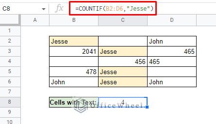
We can even use a cell reference for the condition, and with a little tweaking, make the worksheet more dynamic:

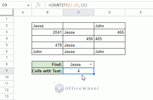
Learn More: COUNTIF Contains Text in Google Sheets (4 Ways)

2. Sum Cells Whose Number Values are Formatted as Text

The case here is slightly different. Here, we want to sum the values of the numbers that are formatted as text in Google Sheets.

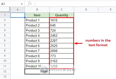
In the image above, we can see that the Quantity values are in the text format. Numbers can be formatted as text manually or it may occur during importing of data. This situation is not uncommon.

But the thing is, when we go to sum these values with the SUM function for the Total, this happens:

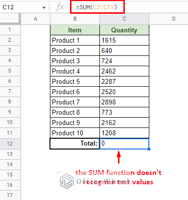
The SUM function doesn’t recognize text values.

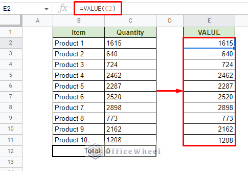
The solution is to extract the underlying number values from the text formatting and then use SUM.

Coincidentally, we have just the function for this: VALUE.

The VALUE function will help extract the original numerical values of the cells. Here’s what happens when we apply it to text numbers:

Now, let’s utilize this function inside SUM to get the total of the Quantities:

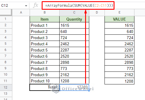
Reason for using ARRAYFORMULA

The VALUE function cannot take a range of cells as an argument. So, we have to present each value of the range as an array. These values are then used by SUM to sum the values as usual.

You can easily apply ARRAYFORMULA by pressing CTRL+SHIFT+ENTER instead of just ENTER after writing =SUM(VALUE(C2:C11)). You can also enclose the formula manually.

3. Sum Cells Depending on Text Value in another Cell

In this example, we want to find the sum of the Quantity depending on the text value in another cell in Google Sheets.

Our worksheet:

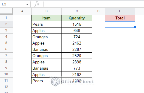
Let’s consider “Apples” to be our text to search for to calculate the total Quantity.

Since it is a sum with a condition, the perfect formula for this scenario is the SUMIF function.

The formula is:

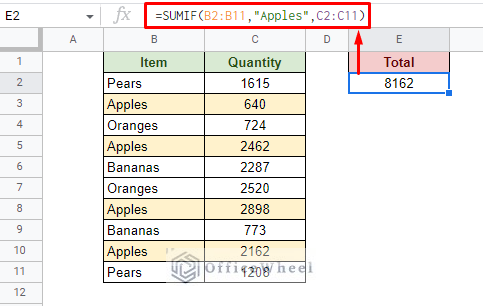
Let’s take things a step further and make the formula more dynamic by adding an item list and a cell reference to it:

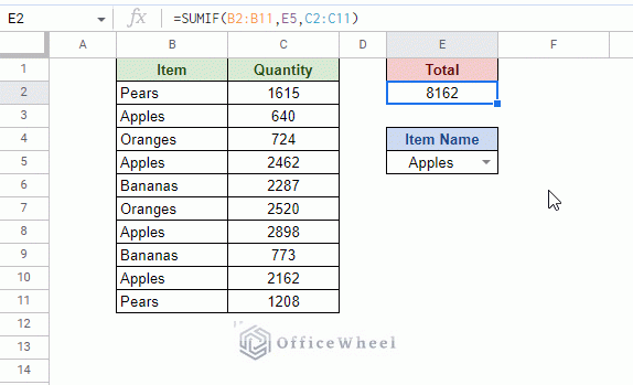
Sum for Cells Containing Partial Text Match

The SUMIF can also be used for partial text matches as well. For example, we want to only sum the cells of the Items with the text code NYC in Google Sheets:

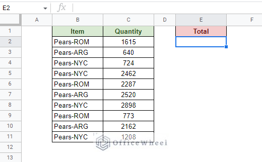
For partial matches, all we have to do is include the asterisk (*) symbol around the condition text.

The formula is:

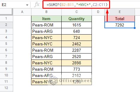
4. Sum Cells with Text and Numbers in the Same Cell in Google Sheets

We may often get number values alongside text in Google Sheets. This is more common when a unit term is attached to a number value. For example, adding “Tons” after a number:

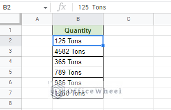
This naturally transforms the value into a text and we will not be able to perform calculations with it.

So, to sum these number value cells with text in Google Sheets, we must extract only the numerical values and then calculate.

We will tell you now that it is not easy and requires a compound function made from the combination of SUM, SPLIT, and REGEXREPLACE as the main functions.

The formula is:

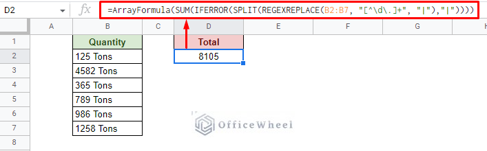
If we want to include the unit:

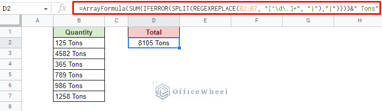
Formula Breakdown

We will start from the middle and move outward:

1. REGEXREPLACE(B2:B7, "[^\d\.]+", "|")

• This replaces all the text values with the pipe (|) symbol. You can use any other symbol here, but we’ve chosen “|” since it is one of the most unused symbols and it is unlikely to naturally appear in a cell.
• The pipe (|) symbol acts as a delimiter that will be used later with the SPLIT function.

2. SPLIT(…,"|")

• Splits the value at the pipe (|) delimiter, essentially extracting the number only from each cell.

3. IFERROR(…)

• Handles any blank cells or errors and returns a blank.

4. SUM(…)

• Sums all the extracted number values by SPLIT.

5. ARRAYFORMULA(…)

• Since we are dealing with multiple (an array) of data, this function allows the formula to handle all of them at once.

Note: This function is only applicable for values in a column arrangement. This shouldn’t be a problem since most data comes in the column arrangement.

Final Words

That concludes the few scenarios on how to sum cells with or depending on the text in Google Sheets.

Most scenarios can be worked with the application of simple functions or functions with conditions attached like SUMIF and COUNTIF. But things can get complex when we have two types of data (number and text) in a single cell.

Feel free to leave any queries or advice you might have for us in the comments section below.

Related Articles for Reading

• How to Perform Conditional Sum in Google Sheets (Easy Guide)
• Applying SUMIF from Another Sheet in Google Sheets
• Count Cells with Color in Google Sheets (3 Easy Ways)
• COUNTIF Multiple Criteria in Google Sheets (3 Ways)
• COUNTIF Across Multiple Sheets in Google Sheets