In business and finance, combining data from multiple columns can be crucial for analysis and decision-making. One way to do this is through the process of concatenating two columns in Google Sheets. For example, by concatenating a column of first names with a column of last names, businesses can create a single column of full names for more efficient customer data management. There are various ways to learn how to concatenate two columns in Google Sheets, and this article aims to provide a comprehensive understanding of the process.
A Sample of Practice Spreadsheet
You can copy our spreadsheet that we’ve used to prepare this article.
2 Ways to Concatenate Two Columns in Google Sheets
Concatenating two columns in Google Sheets is a quick and easy way to combine data from different columns into one. There are two main ways to concatenate columns in Google Sheets: horizontally and vertically.
1. Concatenate Two Columns Horizontally
Concatenating two columns horizontally in Google Sheets allows you to merge the data from two separate columns into one, with the data presented horizontally for each row. This is useful for organizing and formatting your data in a more efficient way.
I. Using ARRAYFORMULA with Ampersand (&)
The ARRAYFORMULA function in Google Sheets is a powerful tool that allows users to apply a single formula to a range of cells with just one input. One way to utilize this function is by combining it with the Ampersand (&) operator.
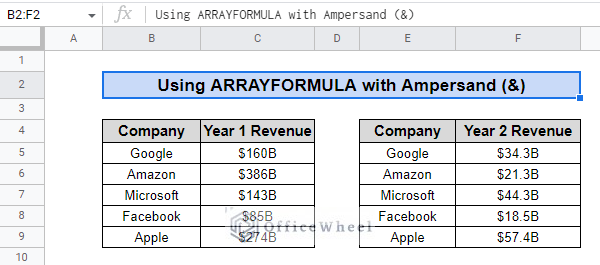
We will use the dataset above to demonstrate the use of ARRAYFORMULA with Ampersand (&) to concatenate two columns.
Steps:
- Firstly, we will select cell C13.
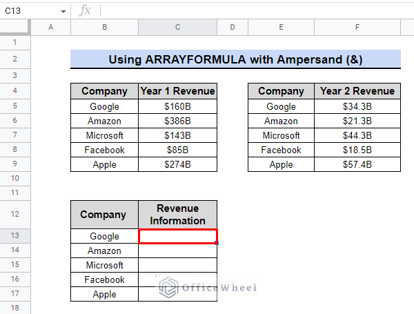
- Secondly, we will use the following formula to combine the data from two columns.
=ARRAYFORMULA({C5:C9&", "&F5:F9})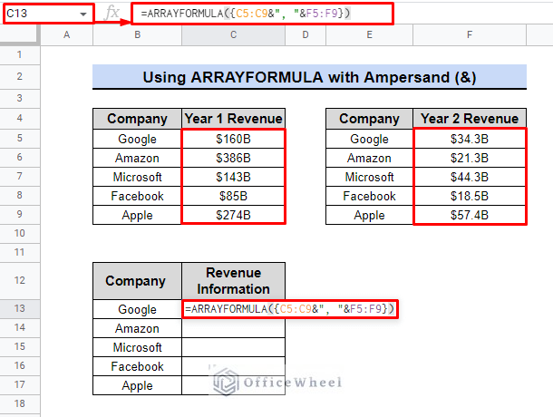
- In this formula, ARRAYFORMULA is being used to apply the Ampersand function to the range of cells C5:C9 and F5:F9.
- This formula will combine the text in the cells in columns C and F, separated by a comma and a space.
- Finally, press ENTER to see the result.
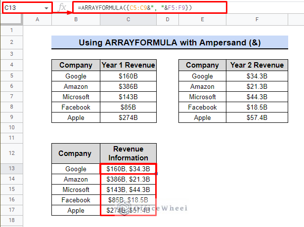
The resulting formula combines the text in the specified ranges with a comma and space in between, creating a concatenated string for each row in the range. The FORMULAARRAY function in combination with the Ampersand (&) symbol is a useful tool for efficiently concatenating multiple cells in a column in Google Sheets.
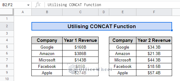
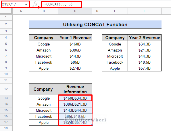
II. Utilizing CONCAT Function
We can combine two strings into a single cell in Google Sheets by using the CONCAT function. Assume that we will use the previous dataset to explain the use of the CONCAT function.
Steps:
- Once again, we will select cell C13.
- We will use the following formula.
=CONCAT(C5,F5)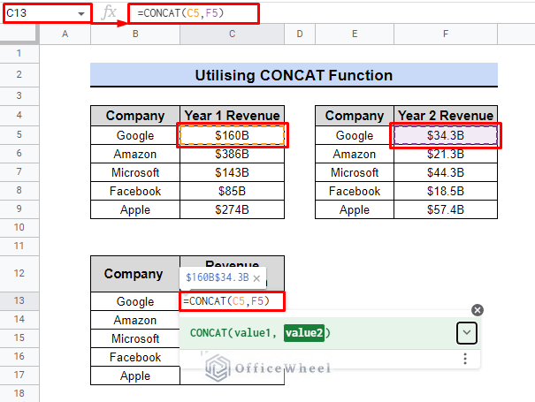
- Combining the text of two or more cells into one cell is one technique to use CONCAT.
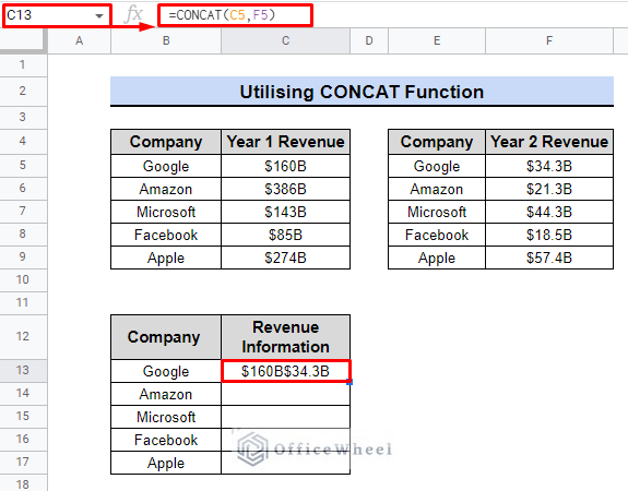
- We shall discover that the CONCAT function will combine the values from cells C5 and F5. As a result, we will discover that Google’s revenue is $160B$34.3B.
- Using the Fill handle feature of google sheets we can get the result of the full Revenue Information column.
III. Utilizing ARRAYFORMULA with CONCAT
We can use the functions ARRAYFORMULA and CONCAT in order to join two columns automatically, without the use of a fill handle. We will use the previous dataset as an example to show the use of these functions.
Steps:
- At first, we are once again going to select cell C13.
- We will use the following formula.
=ARRAYFORMULA(CONCAT(C5:C9,F5:F9))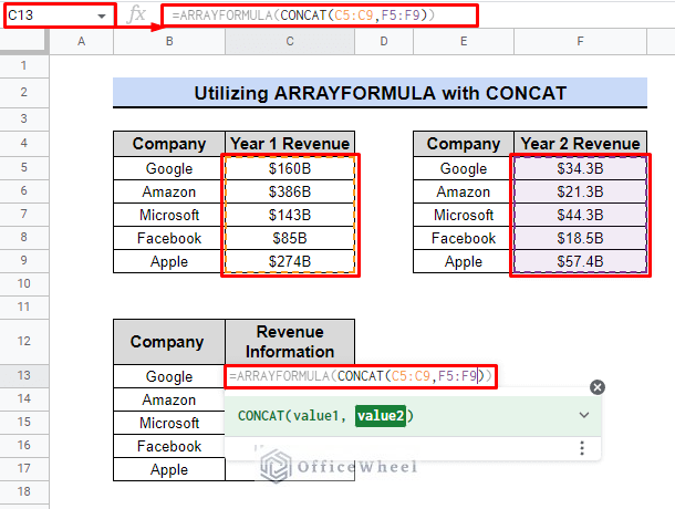
- To conclude, press ENTER.
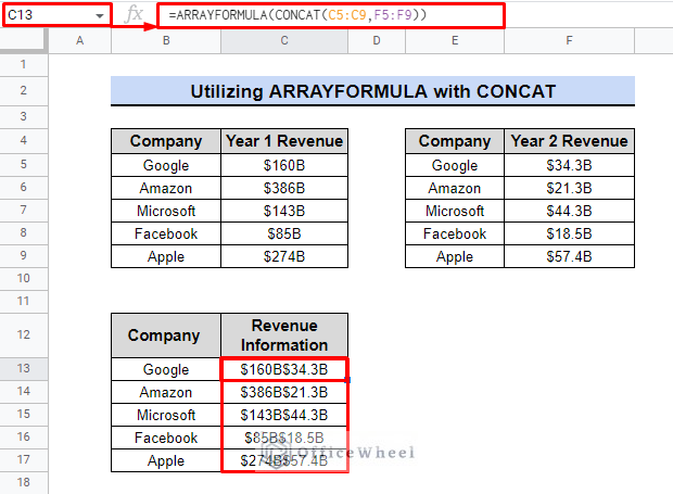
- The CONCAT function returns the concatenation of two ranges from C5:C9 and F5:F9.
- ARRAYFORMULA will then display the value returned by the CONCAT Function in a single array of rows.
Thus, the ARRAYFORMULA and CONCAT functions allow us to combine data from two separate columns into a single column for improved data display.
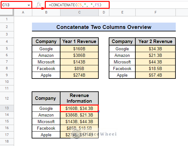
IV. Applying CONCATENATE Function
We can use the CONCATENATE function to combine multiple cells or strings into one cell. We will provide the cell references or strings to be combined as arguments to the function. The following dataset will make a good example to demonstrate the use of the CONCATENATE function.
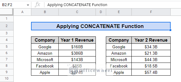
We will make a single column combining the Year 1 and Year 2 Revenue of the companies and rename it into Revenue Information using the following formula.
Steps:
- Let’s select cell C13 first.
- Then we will use the following formula.
=CONCATENATE(C5,", ",F5)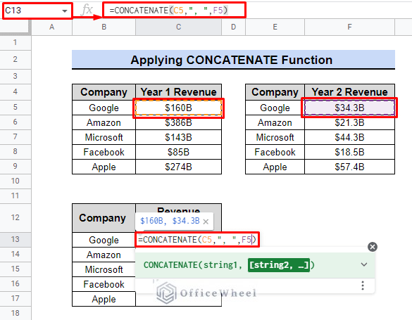
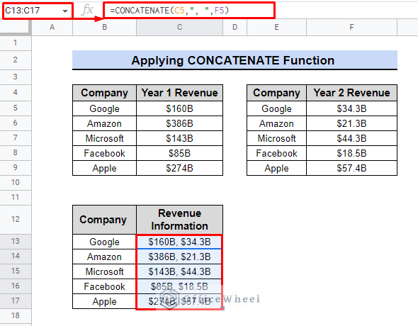
- Now we will use the fill handle feature of google sheets to get results for the rest of the companies.
- The CONCATENATE function starts by taking the text in cell C5.
- Next, it adds a comma and then adds a space, represented by the “, “ in the formula.
- Finally, it adds the text in cell F5.
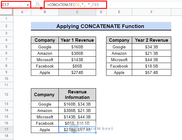
This function helps simplify and combine data, making it easy to view and understand the revenue for two years at a glance.
Read More: How to Concatenate Strings with Separator in Google Sheets
Similar Readings
- How to Append Text in Google Sheets (An Easy Guide)
- Add Space with CONCATENATE in Google Sheets
- How to Concatenate Text and Formula in Google Sheets (7 Ways)
2. Concatenate Two Columns Vertically
Concatenating two columns vertically in Google Sheets can be done using the following methods. This is useful for creating a comprehensive list of items or data points, without the need to manually copy and paste
I. Using Simple Array Reference
Simple array references are a way to reference a group of cells in a worksheet in a single formula. They are created by enclosing a range of cells in curly braces {}. This allows you to quickly reference a range of cells, rather than having to enter each individual cell reference into a formula. This can save time and help make your formulas more organized and easy to read.
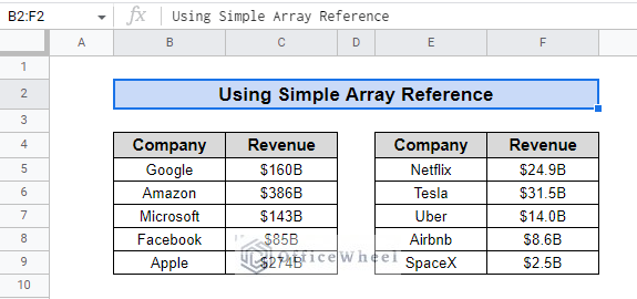
We will be using the above dataset to demonstrate the process.
Steps:
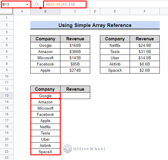
- First, we need to select the cell, for this case, it is B13.
- Later on, we will use the following formula.
={B5:B9;E5:E9}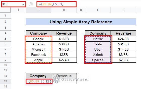
- After pressing ENTER, We will find that it displays the result of the array reference.
- Additionally, We can use this same formula to fill up the Revenue column in by selecting cell C13.
={C5:C9;F5:F9}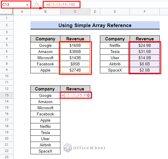
- This formula will create a simple array reference by combining the values of the cells in the range C5 to C9 and F5 to F9, and displaying them in a single array.
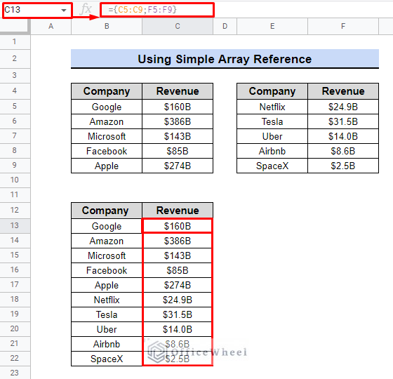
By using the formula, we can now view the total revenue of each company in one table instead of two duplicate tables.
Read More: How to Concatenate If Cell Is Not Blank in Google Sheets (7 Ways)
II. Implementing UNIQUE Function
The UNIQUE function is important for identifying and removing duplicate values in a dataset. It is commonly used to ensure data accuracy and integrity. However, it can also be used to extract distinct values from a combined range of cells.
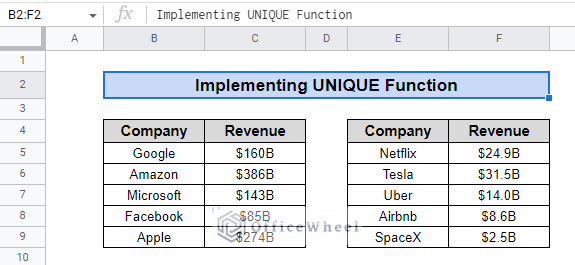
We will be using the above-mentioned dataset to illustrate the use of the UNIQUE function to concatenate two columns in google sheets.
Steps:
- Once again, we will select cell B13 first.
- Now we will use the following formula.
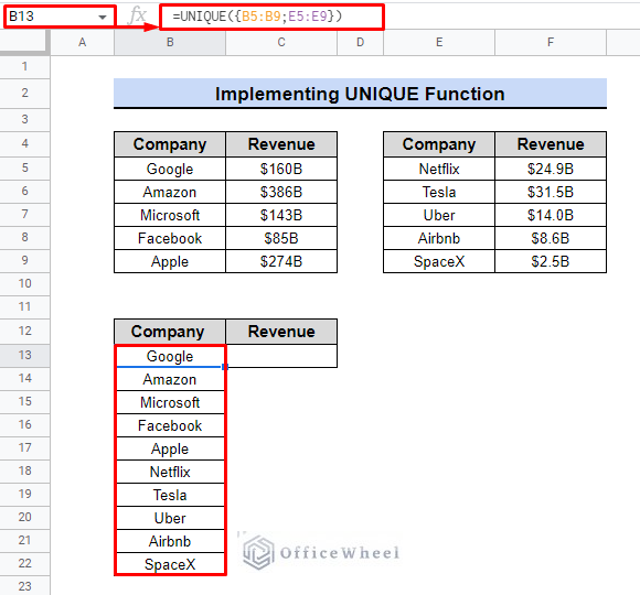
=UNIQUE({B5:B9;E5:E9})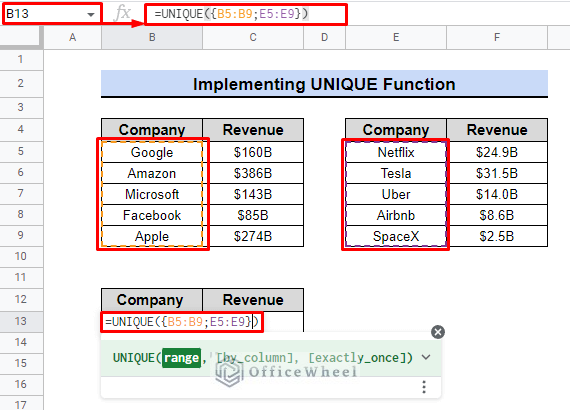
- This formula uses the UNIQUE function to find unique values in two defined ranges of cells C5:C9 and F5:F9 separated by a semicolon (;) using curly braces {} to group cells and use it as a reference. The result will be a list of unique values.
- We will use the following formula in cell C13 to complete the table.
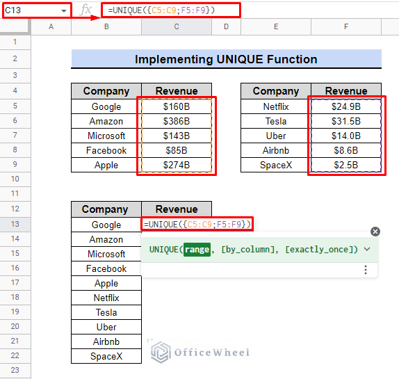
=UNIQUE({C5:C9;F5:F9})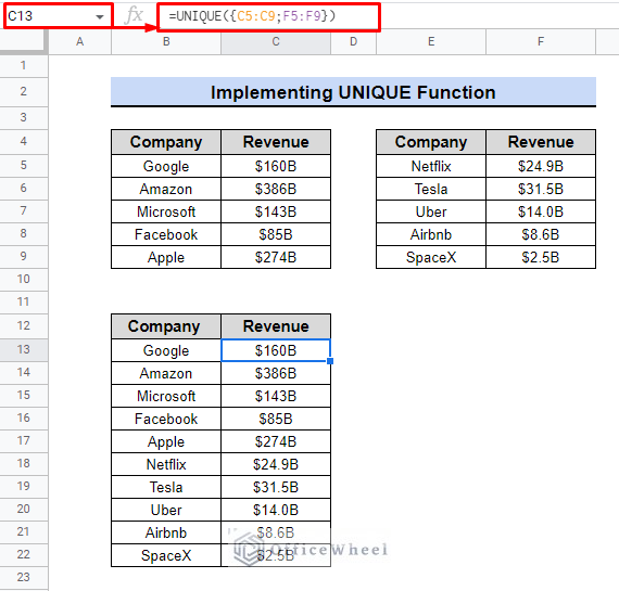
In conclusion, by combining two tables into one and reducing the number of columns, we now have a more organized and efficient way of displaying the companies and their revenues.
Read More: How to Concatenate Values for IF Condition in Google Sheets
III. Combining FILTER and LEN Functions
Efficient data management requires the use of practical tools. FILTER and LEN functions in Google Sheets allow for quick data extraction and validation. Use them to organize and analyze your data effectively.
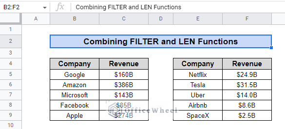
By utilizing the FILTER and LEN functions, we can combine two tables into one using the same dataset.
Steps:
- Once Again, select cell, B13.
- Now, we will use the following formula to list the company names.
=FILTER({B5:B9;E5:E9},LEN({B5:B9;E5:E9}))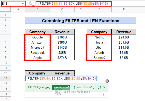
- Inside the FILTER function, the range of cells being filtered is {B5:B9;E5:E9}. This range includes cells B5 through B9 and E5 through E9.
- The condition used to filter the cells is LEN({B5:B9;E5:E9}). LEN function is used to determine the number of characters in a cell or text string.
- By using the LEN function inside the FILTER function, we’re able to filter out cells with a certain number of characters, in this case, it will filter out cells that have no characters or empty cells.
- The final result is a filtered range of cells that contains only cells with character.
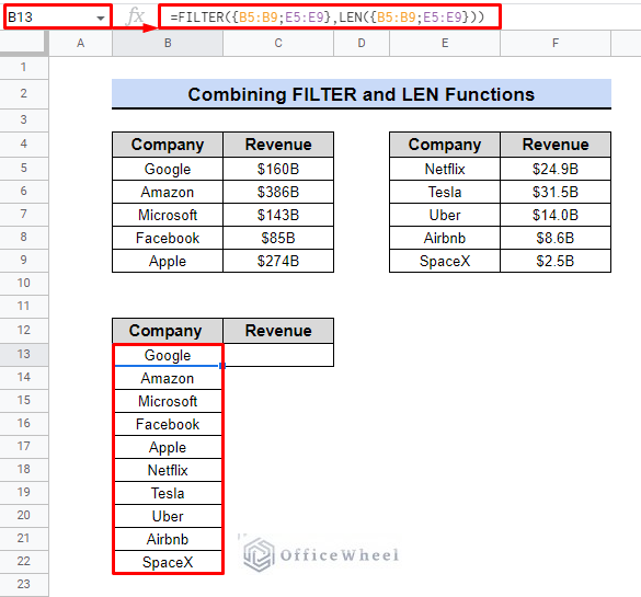
- Next, we will create a list by combining the Revenue columns.
- We will select cell C13 and apply the following formula.
=FILTER({C5:C9;F5:F9},LEN({C5:C9;F5:F9}))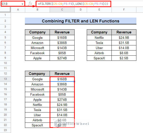
By using the same process and condition, the formula extracts all the revenues of the companies. Therefore, we can use the FILTER and LEN functions to concatenate two columns in Google Sheets.
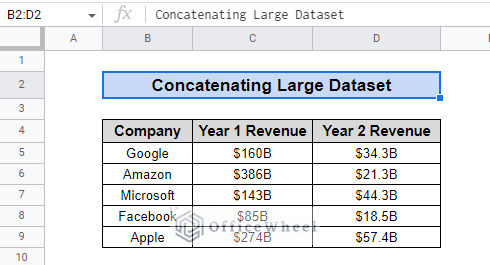
IV. Concatenating Large Dataset with QUERY Function
In Google Sheets, we may concatenate enormous amounts of data over several columns by using the QUERY function. To illustrate how to use this function, we’ll use the subsequent dataset.
Steps:
- The first step is to choose cell B13.
- Next, we’ll combine the TRANSPOSE function with the QUERY function.
=TRANSPOSE(QUERY(TRANSPOSE(B5:D9),,9^9))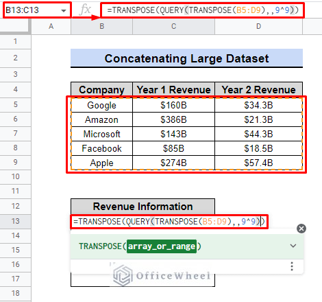
- Finally, press ENTER to see the result.
- The inner TRANSPOSE function swapped the rows and columns of range B5 to D9.
- QUERY function uses the values returned by the TRANSPOSE function as data.
- By choosing 9^9, the header of the data rows for the QUERY function is equivalent to infinite.
- The outer TRANSPOSE function once more reverses the values that the QUERY function returned.
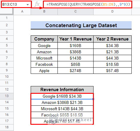
We can see that the formula has concatenated all three adjacent columns.
If the data set is not adjacent to each other, we can use the following formula to concatenate multiple columns.
=TRANSPOSE(QUERY(TRANSPOSE({B5:C9,F5:F9}),,9^9))Read More: Google Sheets QUERY Function to Concatenate Two Columns
Conclusion
By using these functions, data management becomes more efficient as the number of columns is reduced and information is displayed in a more streamlined manner. This approach allows for easy organization and extraction of specific data, leading to better decision-making and improved business performance.
In summary, understanding how to concatenate two columns using these functions can improve organizational efficiency and support economic growth. Check OfficeWheel for more help.