When trying to organize a group of data on a single page, Google Sheets’ ability to combine columns may be quite useful. It can speed up production, save time, and ultimately benefit the person greatly. If we wish to combine two columns in Google Sheets, we can use the QUERY function to do so. In this article, I’ll demonstrate 2 simple ways to use the QUERY function to concatenate two columns in Google Sheets. Here is an overview of what we will archive:
2 Simple Ways to Use QUERY Function to Concatenate Two Columns in Google Sheets
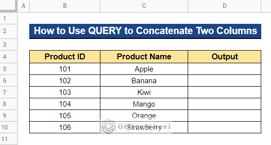
We will use the dataset below to demonstrate 2 simple ways to use the QUERY function to concatenate two columns in Google Sheets. The dataset contains a list of Product IDs and Product Names of a particular shop. Now, we want to combine the two columns in Google Sheets using the QUERY function.
1. Merging TRANSPOSE and QUERY Functions
We can combine the TRANSPOSE and QUERY functions to concatenate two columns in Google Sheets. When applied to any dataset, the QUERY function can run a Google Visualization API Language query, while the TRANSPOSE function can change rows into columns or columns into rows.
Steps:
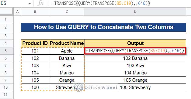
- Firstly, select a cell where you want to apply the formula to combine two columns. In our case, we selected Cell D5. Next, input the formula below and press Enter–
=TRANSPOSE(QUERY(TRANSPOSE(B5:C10),,6^6))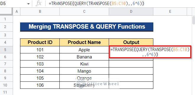
Formula Breakdown
- TRANSPOSE(B5:C10)
First, the given range of Cells B5:C10 is transposed using this TRANSPOSE function.
- QUERY(TRANSPOSE(B5:C10),,6^6)
The QUERY function then does a query over the transposition and returns all entries as no query statement is given. To combine all the cells in a column into a single cell, a high number 6^6 is supplied as the header row count.
- TRANSPOSE(QUERY(TRANSPOSE(B5:C10),,6^6))
The row given by the QUERY function is changed into a column by this TRANSPOSE function.
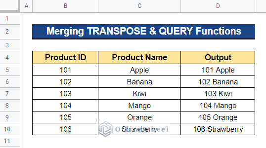
- You will thus receive the concatenation of Column B and Column C along with the space in between them.
2. Joining ARRAYFORMULA, SUBSTITUTE, TRIM, TRANSPOSE, QUERY, and COLUMNS Functions
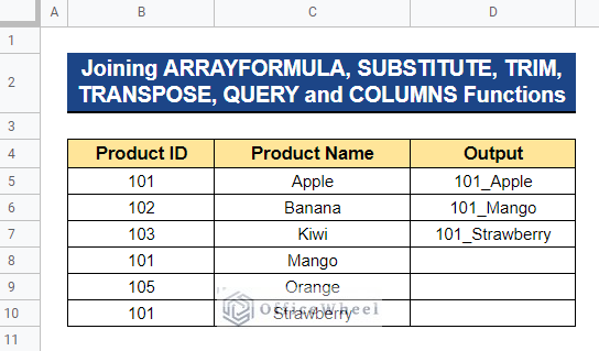
Occasionally, you might wish to concatenate a query’s results in Google Sheets. You can do this by combining the ARRAYFORMULA, SUBSTITUTE, TRIM, TRANSPOSE, QUERY, and COLUMNS functions. Here, we will concatenate Column B and Column C if Column B contains 101 as a Product ID.
Steps:
- To combine two columns depending on a query result, first choose the cell where you wish to apply the formula. In our instance, we decided on Cell D5. Next, type the formula below and press Enter–
=ARRAYFORMULA(SUBSTITUTE(TRIM(TRANSPOSE(QUERY(TRANSPOSE(QUERY(B5:C10, "select * where B contains '101'")),,COLUMNS(QUERY(B5:C10, "select * where B contains '101'")))))," ","_"))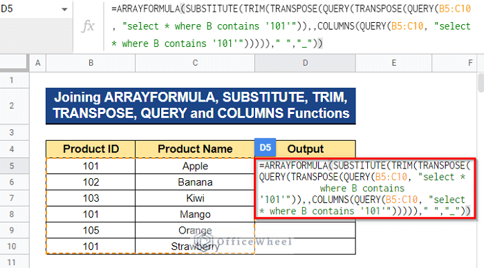
Formula Breakdown
- QUERY(B5:C10, “select * where B contains ‘101’”)
Firstly, the QUERY function does a query and returns all the rows that contain a Product ID of 101 in Column B.
- TRANSPOSE(QUERY(B5:C10, “select * where B contains ‘101’”))
The TRANSPOSE function transposes the rows into columns.
- QUERY(TRANSPOSE(QUERY(B5:C10, “select * where B contains ‘101’”)),,COLUMNS(QUERY(B5:C10, “select * where B contains ‘101’”)))
After that, the QUERY function does a query over the transposition and returns all values that contain 101.
- TRANSPOSE(QUERY(TRANSPOSE(QUERY(B5:C10, “select * where B contains ‘101’”)),,COLUMNS(QUERY(B5:C10, “select * where B contains ‘101’”))))
Afterward, the TRANSPOSE function transposes the results.
- TRIM(TRANSPOSE(QUERY(TRANSPOSE(QUERY(B5:C10, “select * where B contains ‘101’”)),,COLUMNS(QUERY(B5:C10, “select * where B contains ‘101’”)))))
Next, the TRIM function eliminates text’s leading, trailing, and repetitive spaces.
- SUBSTITUTE(TRIM(TRANSPOSE(QUERY(TRANSPOSE(QUERY(B5:C10, “select * where B contains ‘101’”)),,COLUMNS(QUERY(B5:C10, “select * where B contains ‘101’”))))),” “,”_”)
The SUBSTITUTE function then connects the two outputs using an underscore (_) as a separator.
- ARRAYFORMULA(SUBSTITUTE(TRIM(TRANSPOSE(QUERY(TRANSPOSE(QUERY(B5:C10, “select * where B contains ‘101’”)),,COLUMNS(QUERY(B5:C10, “select * where B contains ‘101’”))))),” “,”_”))
Here, the ARRAYFORMULA function returns non-array cells into an array.
- As a result, you will get the concatenation of Column B and Column C based on a query result.
4 Alternatives of Using QUERY Function to Concatenate Two Columns in Google Sheets
To combine two columns in Google Sheets, we don’t always need to utilize the QUERY function. Instead of utilizing the QUERY method to concatenate two columns in Google Sheets, we will utilize 4 alternatives in this case.
1. Using ARRAYFORMULA and Ampersand Operator
In Google Sheets, joining cells together with the ampersand (&) operator is probably the simplest way to concatenate two columns. Using the ampersand operator, we can additionally insert additional delimiters or spaces between the text from each cell. We can execute concatenation operations for a range if we utilize the ARRAYFORMULA function and the ampersand operator. We won’t need to utilize the Fill Handle icon as a result.
Steps:
- First, choose the cell to which you’ll be applying the formula to join two columns. In this instance, we chose Cell D5. Next, enter the following formula and hit Enter–
=ARRAYFORMULA(B5:B10&""&C5:C10)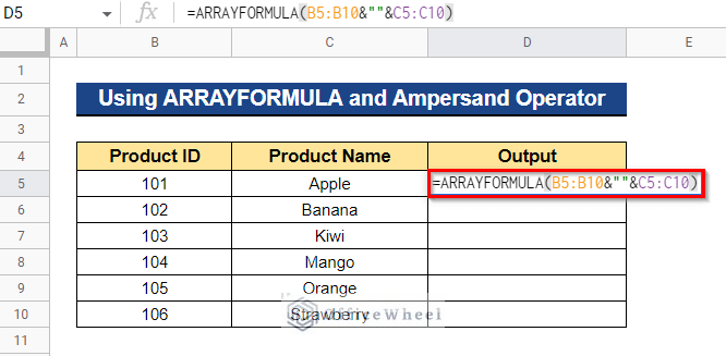
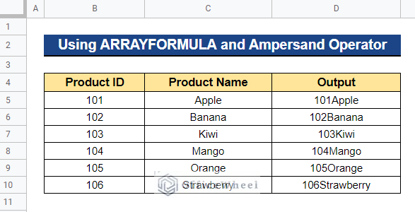
- Thus, you will get the result of concatenating Column B and Column C.
Read More: How to Concatenate Text and Formula in Google Sheets (7 Ways)
2. Combining IF and CONCATENATE Functions
In Google Sheets, we may occasionally want to combine two columns depending on specified criteria. Here, we’ll combine only the products which have the corresponding ID- 101. By combining the IF function with the CONCATENATE function, we can conduct conditional concatenation activities. Moreover, if you want to utilize this method for a range, you have to utilize the Fill Handle icon to do so.
Steps:
- Choose a cell to apply the formula to in order to merge two columns. In our instance, we decided on Cell D5. Next, enter the following formula and hit Enter–
=IF(B5<>101,"",CONCATENATE(B5," ",C5))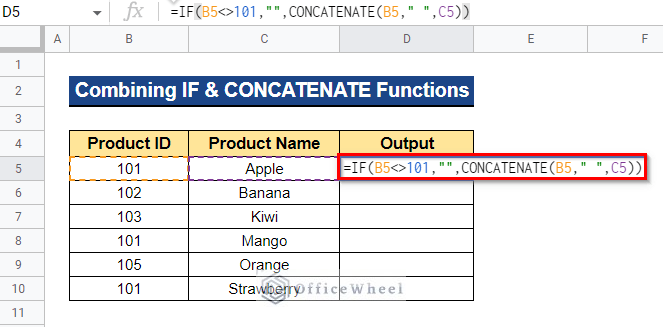
Formula Breakdown
- CONCATENATE(B5,” “,C5)
Firstly, the CONCATENATE function connects Cell B5 and Cell C5 with a space in between them.
- IF(B5<>101,””,CONCATENATE(B5,” “,C5))
Then, the IF function will return a blank cell if Cell B5 doesn’t contain 101 as a Product ID. Otherwise, it will return the output of the CONCATENATE function.
- Now, to apply the formula to the remaining cells, drag the Fill Handle icon downward.
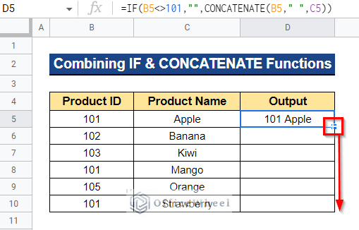
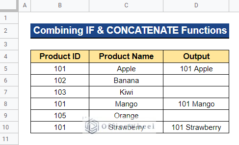
- Therefore, if Column B has a Product ID of 101, you will get the concatenation of Column B and Column C. Otherwise, you will get a blank cell as an output.
Similar Readings
- How to Concatenate Strings in Google Sheets (2 Easy Ways)
- How to Concatenate With Separator in Google Sheets (3 Ways)
- How to Append Text in Google Sheets (An Easy Guide)
3. Applying CONCATENATE Function
Concatenating two columns in Google Sheets is also possible by using the CONCATENATE function. Additionally, we may use the CONCATENATE function to insert additional delimiters or spaces between the text from each cell.
Steps:
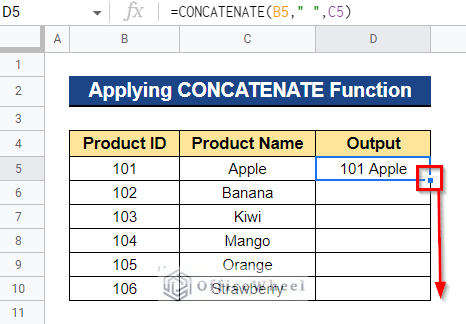
- In order to combine two columns, you must first choose the cell where the formula will be applied. We chose Cell D5 in our instance. Next, input the formula below and hit Enter–
=CONCATENATE(B5," ",C5)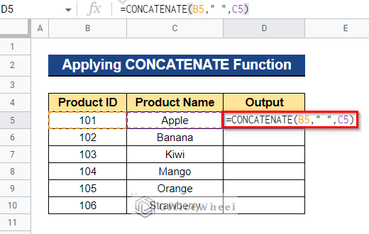
- Now, drag the Fill Handle symbol downward to apply the formula to the remaining cells.
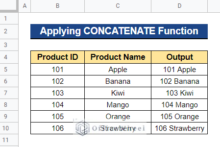
- As a result, you will obtain Column B and Column C combined.
Read More: How to Concatenate in Google Sheets (6 Suitable Ways)
4. Merging ARRAYFORMULA and CONCAT Functions
To conduct concatenation operations for a whole column, we may also connect the ARRAYFORMULA function with the CONCAT function. The CONCAT function has the restriction that strings from two cells cannot have spaces or delimiters between them.
Steps:
- First, choose the cell to which you wish to apply the formula to merge two columns. In our situation, we chose Cell D5. After that, enter the formula below and hit Enter–
=ARRAYFORMULA(CONCAT(B5:B10,C5:C10))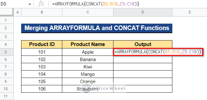
Formula Breakdown
- CONCAT(B5:B10,C5:C10)
For the two values in the given range, the CONCAT function executes a combination operation.
- ARRAYFORMULA(CONCAT(B5:B10,C5:C10))
Here, the CONCAT function receives assistance from the ARRAYFORMULA function to handle an array and show the outcome as an array.
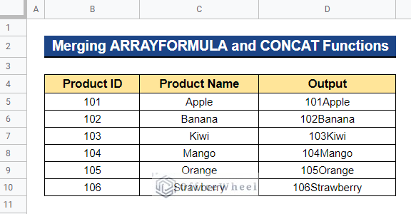
- As a result, you will obtain Column B and Column C combined with no spaces between them.
Read More: How to Add Space with CONCATENATE in Google Sheets
Conclusion
This completes our tutorial on utilizing Google Sheets’ QUERY function to concatenate two columns. I hope the examples I gave would satisfy your requirements. Alternatives to the QUERY function that we explained in this post are also available. Please use the comment section to share your opinions on the article. For more informative articles about Google Sheets, visit our website Officewheel.com.
Related Articles
- How to Concatenate Number and String in Google Sheets
- Concatenate Multiple Cells in Google Sheets (11 Examples)
- How to Concatenate If Cell Is Not Blank in Google Sheets (7 Ways)
- Concatenate Strings with Separator in Google Sheets
- How to Concatenate Double Quotes in Google Sheets (3 Ways)
- Get Opposite of Concatenate in Google Sheets (2 Ways)
- How to Concatenate Values for IF Condition in Google Sheets