We often need to split a large text string and rearrange them within different columns. Like, if a company has a dataset that contains information on all the employees including their full names and then if they want to make a new dataset containing the whole information with first name and last name separately instead of full names, what will they do? Will they start typing the whole thing in a new worksheet? Or will they copy and paste them one by one? Definitely not. The use of built in QUERY function with SPLIT function in Google Sheets really works in an amazing way for that. There are various uses for these two functions together. One of the outputs is as follows.

A Sample of Practice Spreadsheet
You can download the spreadsheet used for describing methods in this article from here.
5 Quick Methods to Use QUERY with SPLIT Function in Google Sheets
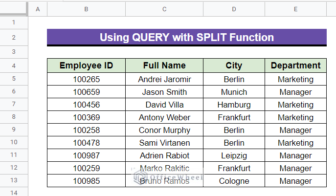
We will be using the following sample dataset for explaining the methods in this article. The dataset contains some employees’ information about a company.
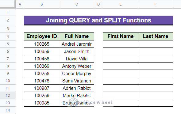
1. Joining QUERY and SPLIT Functions
Suppose, in the following worksheet below, we want to separate the first and last names of each employee. We will learn this in a way so that we can separate only the first or the last name if we want. The SPLIT function usually separates both and returns them into two different columns. But with the help of the QUERY function, we can separate them one by one.
Steps:
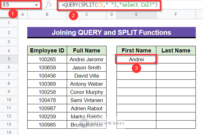
- First, select Cell E5, apply the following formula below and press Enter–
=QUERY(SPLIT(C5," "),"select Col1")The output will be as follows. Here, you can see that the formula returns only the first name as output.
Formula Breakdown
- SPLIT(C5,” “)
First, the SPLIT function will split the text string that is in Cell C5 and the delimiter here is the space which is mentioned as “ ”.
- QUERY(SPLIT(C5,” “),”select Col1”)
Thereafter, the QUERY function will pick the first separated value after the whole text string of Cell C5 is separated by the SPLIT function. The command is given here by “select Col1”.
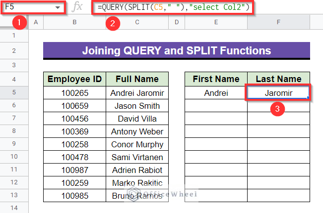
- Now, select Cell F5, insert the following formula and press Enter–
=QUERY(SPLIT(C5," "),"select Col2")The output you will get will be like below. Here, the whole function returns only the last name as output.
Formula Breakdown
- SPLIT(C5,” “)
First, the SPLIT function will split the text string that is in Cell C5 as mentioned previously and the delimiter here is the space that is mentioned as “ ”.
- QUERY(SPLIT(C5,” “),”select Col2”)
After that, the QUERY function will pick the second separated value after the whole text string of Cell C5 is separated by the SPLIT function. The command is given here by “select Col2”.
- After that, select Cell E5 again, and drag down using the Fill handle icon as shown in the circled portion.
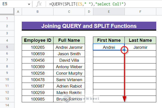
- Following this, the first name of other employees will be separated as follows.
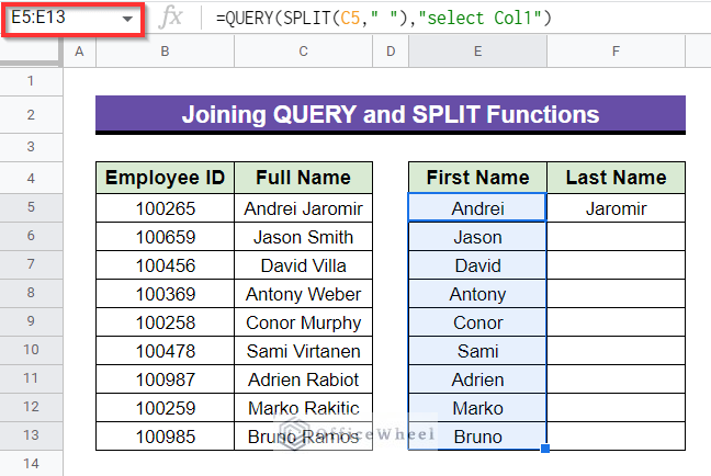
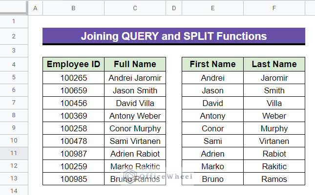
- Do the exact same dragging down with Fill handle icon selecting Cell F5 like previously.
- Finally, the whole output will be as follows.
Read More: How to Split Cells to Get Last Value in Google Sheets (4 Methods)
2. Merging QUERY, ARRAYFORMULA and SPLIT Functions
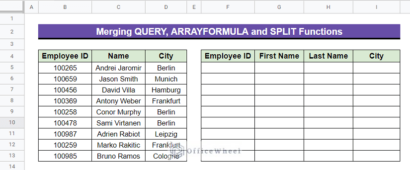
Assume, we want to separate the first and last name of each employee from the following spreadsheet and make another dataset containing all the columns including first and last names columns. A combination of QUERY, ARRAYFORMULA and SPLIT functions will help us with that.
Steps:
- Activate Cell F5, insert the formula below and press Enter–
=QUERY({B5:B13,ARRAYFORMULA(SPLIT(C5:C13," ")),D5:D13},"Select * Where Col1 is not null",1)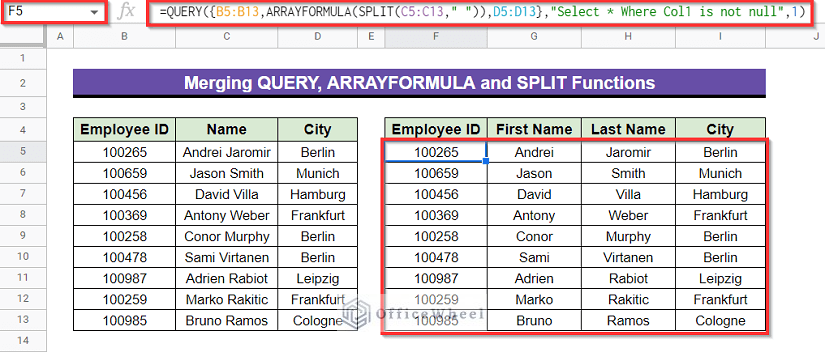
Formula Breakdown
- SPLIT(C5:C13,” “)
First, this function will separate the text strings that are within Cell range C5:C13.
- ARRAYFORMULA(SPLIT(C5:C13,” “))
Then the ARRAYFORMULA applies the SPLIT function to every cell in the predefined range of cells.
- QUERY({B5:B13,ARRAYFORMULA(SPLIT(C5:C13,” “)),D5:D13},”Select * Where Col1 is not null”,1)
Finally, the QUERY function here will pick the previous whole dataset and will make a new one where both the first and last name columns will be new.
Read More: How to Split String into Array in Google Sheets (3 Easy Methods)
Similar Readings
- How to Split View in Google Sheets (2 Easy Ways)
- [Solved!] Split Text to Columns Is Not Working in Google Sheets
- How to Split Address in Google Sheets (3 Easy Methods)
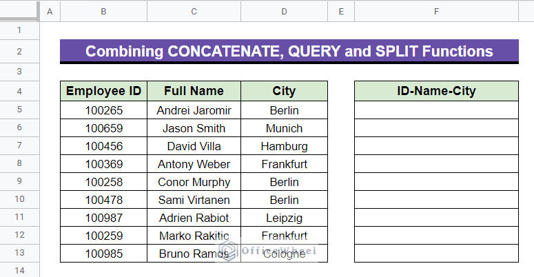
3. Combining CONCATENATE, QUERY and SPLIT Functions
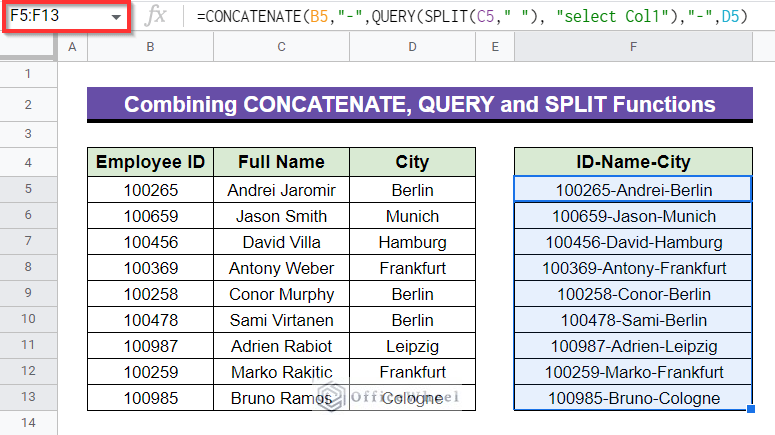
Presume, in the following worksheet, we want to express the employee id, first name of each employee and their corresponding city together in one column. The CONCATENATE function will help to express them like that.
Steps:
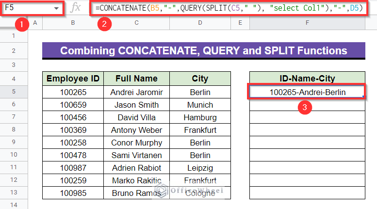
- First, pick Cell F4 in the following dataset, apply the following formula below and press Enter–
=CONCATENATE(B5,"-",QUERY(SPLIT(C5," "), "select Col1"),"-",D5)Following this, the employee id from Cell B5, the first name of employee from Cell C5 and his corresponding city name from Cell D5 will appear as output as follows-
Formula Breakdown
- SPLIT(C5,” “)
First, the SPLIT formula will split the text string that is in Cell C5 and the delimiter here is the space which is mentioned as “ ”.
- QUERY(SPLIT(C5,” “), “select Col1”)
After that, the QUERY function will pick the first separated value after the whole text string of Cell C5 is separated by the SPLIT function as we wanted the first name to appear only. The command is given here by “select Col1”.
- CONCATENATE(B5,”-“,QUERY(SPLIT(C5,” “), “select Col1″),”-“,D5)
Lastly, the CONCATENATE function will concatenate the text in Cell B5, the splitted first name and the text in Cell D5 together.
- Now, drag down using the Fill handle icon as shown in the circled portion.
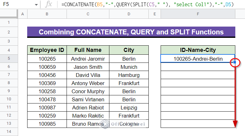
- Lastly, you will get the same output for all other employees as well and the output will be all along in Cell range F5:F13.
Read More: How to Split a Cell in Google Sheets (9 Quick Methods)
4. Merging ARRAYFORMULA, TRIM, SPLIT, TRANSPOSE, QUERY, IF, MOD and ROW Functions
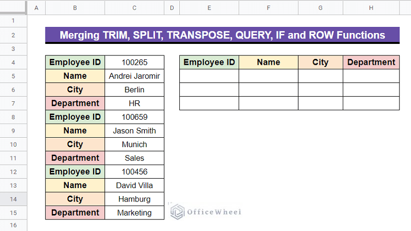
In the spreadsheet below, we can see that the info for each employee is arranged vertically along in only one Column C which can result in procrastination while visualizing them. So what we want to do is rearrange them horizontally along row using the ARRAYFORMULA, TRIM, SPLIT, TRANSPOSE, QUERY, IF, MOD and ROW Functions.
Step:
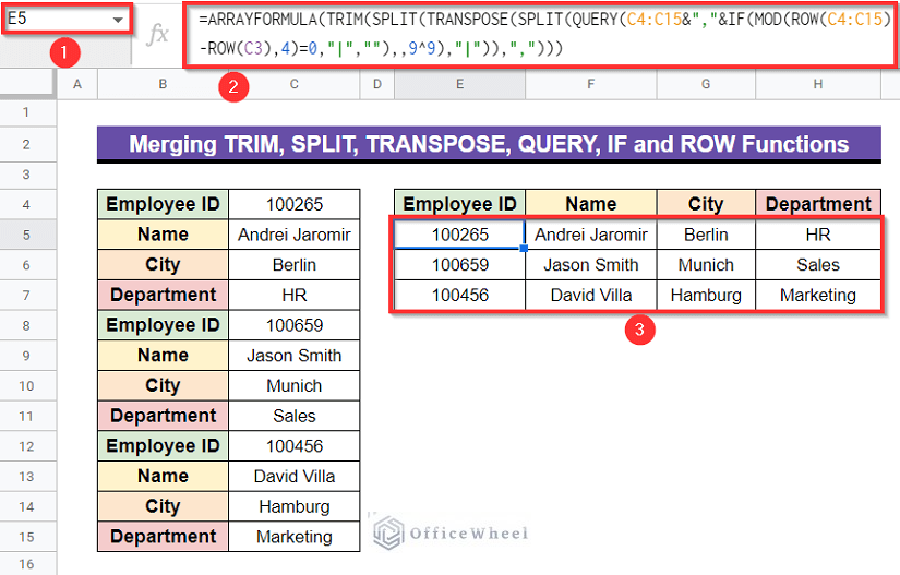
- Select Cell E5, then apply the formula below and press Enter–
=ARRAYFORMULA(TRIM(SPLIT(TRANSPOSE(SPLIT(QUERY(C4:C15&","&IF(MOD(ROW(C4:C15)-ROW(C3),4)=0,"|",""),,9^9),"|")),",")))The final output will be as follows.
Formula Breakdown
- MOD(ROW(C4:C15)-ROW(C3),4)
First, the whole formula will return output “1” for the Cell range C4:C15 which is arranged as 3*4 order.
- IF(MOD(ROW(C4:C15)-ROW(C3),4)=0,”|”,””)
Next, If a logical expression is true, the IF function returns one value; if false, it returns a different value.
- QUERY(C4:C15&”,”&IF(MOD(ROW(C4:C15)-ROW(C3),4)=0,”|”,””),,9^9)
Then, the QUERY function executes queries defined in the SQL.
- SPLIT(QUERY(C4:C15&”,”&IF(MOD(ROW(C4:C15)-ROW(C3),4)=0,”|”,””),,9^9),”|”)
After that, the SPLIT function arranges the whole data into different cells according to the given command.
- TRANSPOSE(SPLIT(QUERY(C4:C15&”,”&IF(MOD(ROW(C4:C15)-ROW(C3),4)=0,”|”,””),,9^9),”|”))
Thereafter, the TRANSPOSE function arranges the vertically arranged data along Column C horizontally.
- SPLIT(TRANSPOSE(SPLIT(QUERY(C4:C15&”,”&IF(MOD(ROW(C4:C15)-ROW(C3),4)=0,”|”,””),,9^9),”|”)),”,”)
Then, the SPLIT formula will split the horizontally arranged data into 3*4 ordered cells.
- TRIM(SPLIT(TRANSPOSE(SPLIT(QUERY(C4:C15&”,”&IF(MOD(ROW(C4:C15)-ROW(C3),4)=0,”|”,””),,9^9),”|”)),”,”))
Next, the TRIM function will remove extra spaces if there are any.
- ARRAYFORMULA(TRIM(SPLIT(TRANSPOSE(SPLIT(QUERY(C4:C15&”,”&IF(MOD(ROW(C4:C15)-ROW(C3),4)=0,”|”,””),,9^9),”|”)),”,”)))
Finally, the ARRAYFORMULA applies the whole function to every cell in the predefined range of cells.
Read More: How to Split Text to Columns Using Formula in Google Sheets
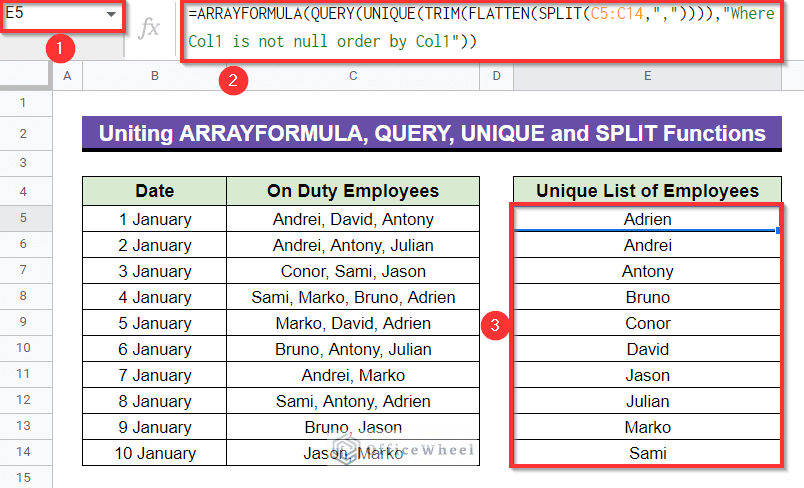
5. Uniting ARRAYFORMULA, QUERY, UNIQUE,TRIM, FLATTEN and SPLIT Functions
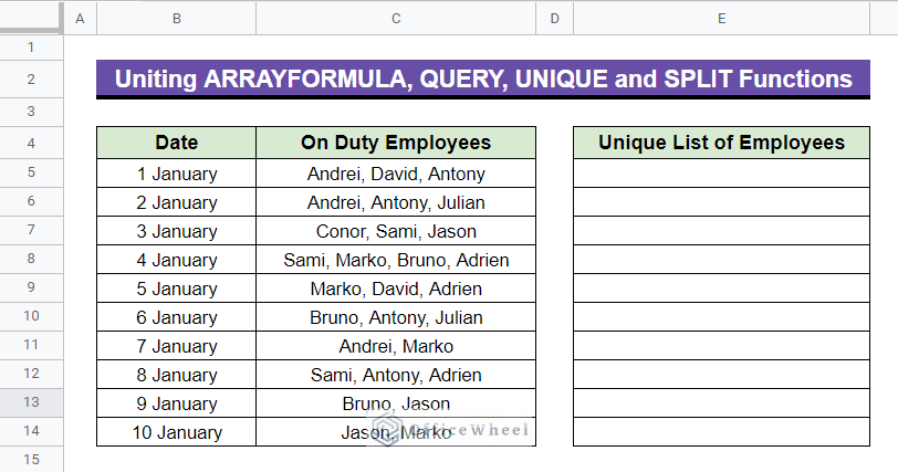
From the following dataset below, what we want to get is a unique list of all the employees who were on duty within the period 1 to 10 January. Combination of some Google sheets built-in functions such as UNIQUE, QUERY, SPLIT, FLATTEN and some other functions will help us to get the unique list in a garnish way.
Steps:
- Choose Cell E5, then insert the formula given below and press Enter–
=ARRAYFORMULA(QUERY(UNIQUE(TRIM(FLATTEN(SPLIT(C5:C14,",")))),"Where Col1 is not null order by Col1"))The result will be as satisfying as follows-
Formula Breakdown
- SPLIT(C5:C14,”,”)
Firstly, the SPLIT function will separate texts that are within Cell range C5:C14. The delimiter here in each cell is a comma “,”.
- FLATTEN(SPLIT(C5:C14,”,”))
Then the FLATTEN formula here will rearrange those separated texts vertically along cells in column E.
- TRIM(FLATTEN(SPLIT(C5:C14,”,”)))
The TRIM function here will eliminate extra spaces if there are any.
- UNIQUE(TRIM(FLATTEN(SPLIT(C5:C14,”,”))))
Next, the UNIQUE function will pick only the unique values from all the texts extracted by the previous formulas.
- QUERY(UNIQUE(TRIM(FLATTEN(SPLIT(C5:C14,”,”)))),”Where Col1 is not null order by Col1″)
After that, the QUERY function will work following the given query “Where Col1 is not null order by Col1”.
- ARRAYFORMULA(QUERY(UNIQUE(TRIM(FLATTEN(SPLIT(C5:C14,”,”)))),”Where Col1 is not null order by Col1″))
Finally, the ARRAYFORMULA applies the whole functions to every cell in the predefined range of cells.
Read More: How to Split Cell by Comma in Google Sheets (2 Easy Methods)
Conclusion
This article contains the 5 easiest and quickest Methods to use QUERY with SPLIT Function in Google Sheets. Hope, this will definitely help you with your task. Visit our site officewheel.com to see more related articles.