In Google Sheets, you can combine cells by using some functions. CONCATENATE, JOIN and TEXTJOIN are the most popular among them. To apply some conditions with the combination you can add the IF and QUERY functions. In this article, we will discuss CONCATENATE IF in Google Sheets which can make your work easier.
A Sample of Practice Spreadsheet
You can download the practice spreadsheet from the download button below.
3 Ways to Concatenate Values for IF Condition in Google Sheets
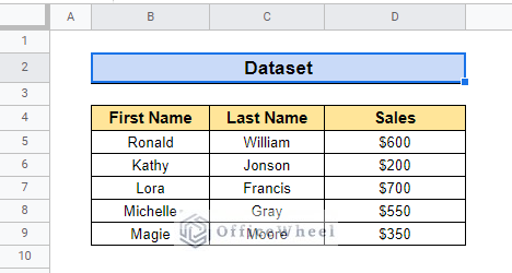
There are three ways to concatenate values for the IF condition in Google Sheets. To show the methods we develop a dataset that contains columns: First Name, Last Name & Sales.
1. Inserting CONCATENATE and IF Functions
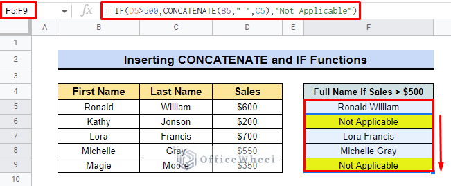
You can use the CONCATENATE and IF functions combined. In that case, the CONCATENATE function will use as the value_if argument of the IF function. So, to apply the method,
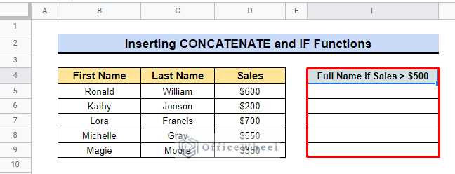
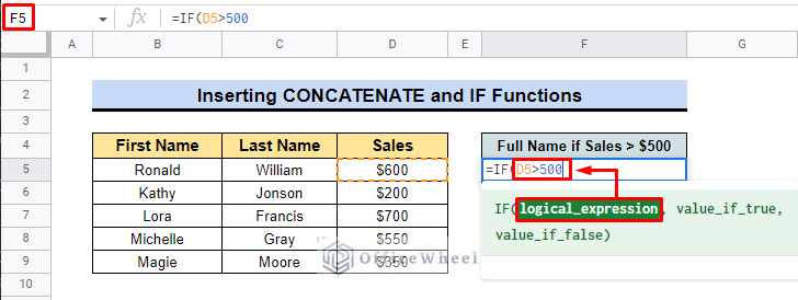
- First, create a result column where we want to show the Full Name if Sales > $500.
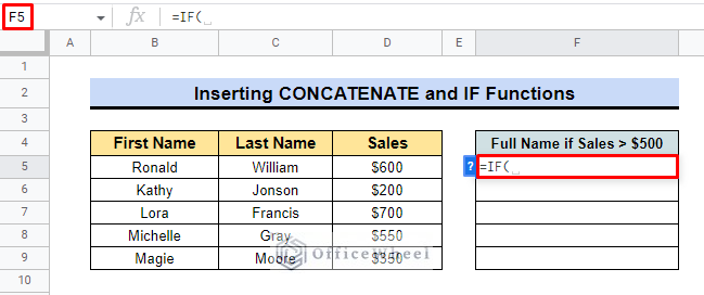
- Then select cell F5 and insert the IF function.
- Now add the logical_expression for the function Here, as we want to show the name whose sales are up to $500 so we add D5>500.D5 represents the first sales cell.
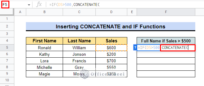
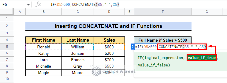
- After that, input the CONCATENATE function as a value_if_true argument.
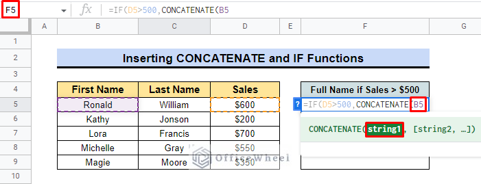
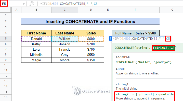
- Now, add the first string of the CONCATENATE function. Here, we add B5 as string1.
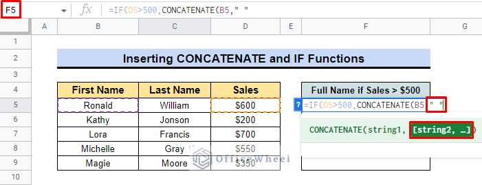
- In the next step, add a space as sting2. To add space, we use the symbol “ “.
- We also add another string which is cell C5. For CONCATENATE function you can add as many strings as you want.
- Now we close the bracket for the CONCATENATE function and its uses as the value_if_true argument for the IF function.
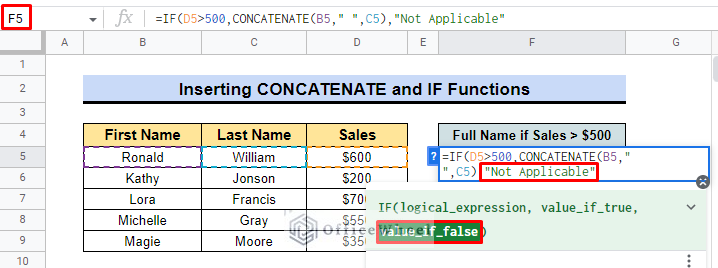
- For the value_if_false parameter, we input a text to specify the values. Here we write down “Not Applicable”.
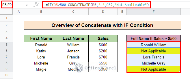
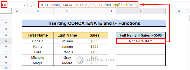
- In the end, press ENTER to apply the function and you will find the desired value in the selected cell.
=IF(D5>500,CONCATENATE(B5,” “,C5),”Not Applicable”)- Finally, you can drag down the Fill handle to apply the function to the entire column and you will find the “Not Applicable” quote where the sales in less than 500.
Read More: How to Concatenate If Cell Is Not Blank in Google Sheets (7 Ways)
Alternative Approach with ARRAYFORMULA
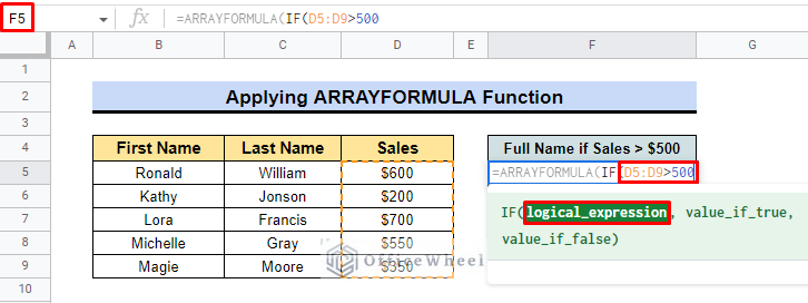
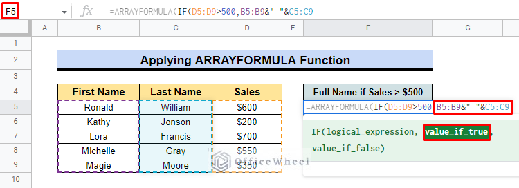
You can apply this same IF conditions for the ARRAY FORMULA function. But the difference between these two methods is here we do not use the CONCATENATE function for linking. Instead of that we just use the ‘&’ symbol to connect cells. To do so,
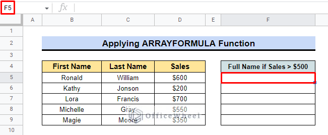
- First Create the same result column Full Name if Sales>$500 and select cell F5.
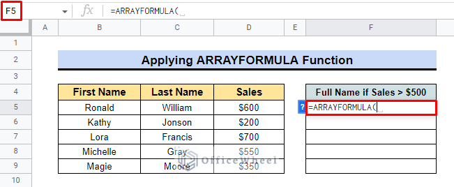
- Then apply the ARRRAYFORMULA function.
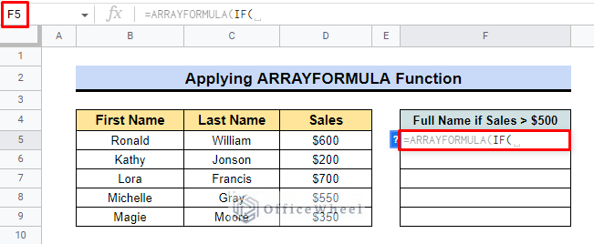
- Then insert the IF function in the cell.
- After that add D5:D9>500 as logical_expression.
- Then input the B5:B9&” “&C5:C9 as value_if_true parameter. Using this, we’ll not require the CONCATENATE function.
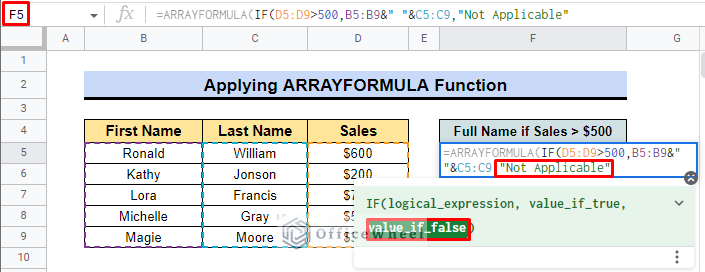
- Then insert the sentence “Not Applicable” as the value_if_false argument.
- Finally, press ENTER to apply the function.
=ARRAYFORMULA(IF(D5:D9>500,B5:B9&” “&C5:C9,”Not Applicable”))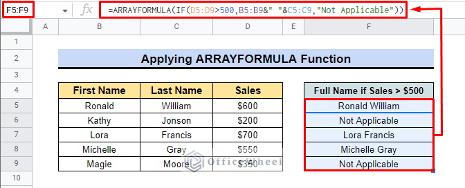
Read More: How to Concatenate Text and Formula in Google Sheets (7 Ways)
Similar Readings
- How to Concatenate in Google Sheets (6 Suitable Ways)
- Concatenate Double Quotes in Google Sheets (3 Ways)
- How to Concatenate Strings in Google Sheets (2 Easy Ways)
2. Using QUERY Formula
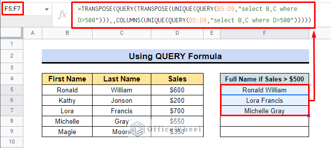
If you want to extract only the names that fulfill the conditions, then you can apply the QUERY formula.
For the QUERY formula, you can use the same dataset and can extract the Full Name if Sales >500.
To do so, you have to insert the following complex formula with QUERY formula in cell F5 and extract the desired results in the entire column F5:F9.
=TRANSPOSE(QUERY(TRANSPOSE(UNIQUE(QUERY(B5:D9,"select B,C where D>500"))),,COLUMNS(UNIQUE(QUERY(B5:D9,"select B,C where D>500")))))Formula Breakdown
- QUERY(B5:D9,“select B,C where D>500”): Returns values from columns B and C that match the condition “>500” in column D.
- UNIQUE(QUERY(B5:D9,“select B,C where D>500”)): Outputs only unique values from the query.
- TRANSPOSE(UNIQUE(QUERY(B5:D9,“select B,C where D>500”))): Used as the range of the QUERY formula.
- COLUMNS(UNIQUE(QUERY(B5:D9,“select B,C where D>500”))): Represents headers.
- ,,: The empty query field returns all applicable data.
- TRANSPOSE(QUERY(TRANSPOSE(UNIQUE(QUERY(B5:D9,“select B,C where D>500”))),,COLUMNS(UNIQUE(QUERY(B5:D9,“select B,C where D>500”))))): transposes all the results to be presented as individual rows, otherwise all the results would have been presented in a single row.
Read More: Google Sheets QUERY Function to Concatenate Two Columns
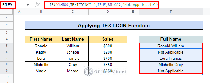
3. Applying TEXTJOIN Function
To link the first and last name you can also apply the TEXTJOIN function. It is the alternative to the CONCATENATE function.
After applying the function in cell F5, we will find the following output,
=IF(D5>500,TEXTJOIN(“ “,TRUE,B5,C5), “Not Applicable”)Formula Breakdown
- TEXTJOIN(“ “,TRUE,B5,C5): join the cell B5 and C5.
- D5>500: represents the value that exceeds sales of $500.
- IF(D5>500,TEXTJOIN(“ “,TRUE,B5,C5), “Not Applicable”): It present two conditions. For TRUE argument it returns the full name or for FALSE it returns the “Not Applicable” text.
Read More: How to Append Text in Google Sheets (An Easy Guide)
Things to Remember
- Always use double quotations to add any type of text.
- Insert the range carefully.
- Use the fill handle to apply the function to the entire column.
Conclusion
We believe this article will help you to understand how to concatenate values for IF condition in Google Sheets. To explore more about Google Sheets, visit the OfficeWheel website.
Related Articles
- How to Concatenate Two Columns in Google Sheets
- Concatenate Strings with Separator in Google Sheets
- How to Add Space with CONCATENATE in Google Sheets
- Concatenate With Separator in Google Sheets (3 Ways)
- How to Concatenate Number and String in Google Sheets
- Get Opposite of Concatenate in Google Sheets (2 Ways)

