
Today, we look at how to reference another sheet in Google Sheets. While it does sound easy (and it is), it’s common to see users of all levels of spreadsheet ...

Today, we will look at the use of INDEX MATCH in Google Sheets. This amazing combination of functions is available in both Excel and Google Sheets. So, if you ...

In this article today, we will be looking at a few ways to compare two columns in Google Sheets. Most of our methods are an iteration of the base, modified ...

Find and Replace is an indispensable tool provided by Google Sheets. If you are thinking of the simple Find option, then you couldn’t be further away from the ...

In professional work, we are often asked to tackle worksheets that have large amounts of data. In such cases, it is imperative that we freeze up our table ...

In today’s article, we will be looking at how to freeze columns in Google Sheets. Know that the processes are basic and can be used by users of any level of ...

Whether it be personal or for data cleanup and organization reasons, knowing how to unmerge cells in Google Sheets is crucial. And that is exactly what we ...

Sometimes, the traditional ways to merge cells in google sheets may not cut it, thanks to the wiping of data that happens with the built-in function. For ...

Knowing how to merge columns in Google Sheets is a fairly easy affair. But things can get complicated when a lot of data and specific criteria are involved. ...

Merging cells is one of the core functions of any spreadsheet application. Not only for organizing data, cell merges can also be utilized to make your ...

In this article, we will learn how to wrap text in Google Sheets, which is one of the fundamental functions of the application. 4 Ways to Wrap Text in Google ...
As complex as custom formulas can be, they are a lifesaver when working with spreadsheets that contain large amounts of data. On the other hand, you have a ...
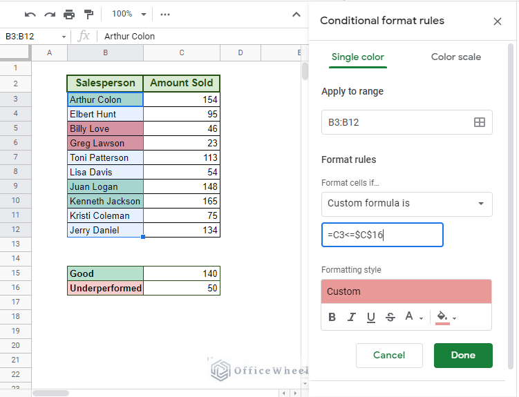
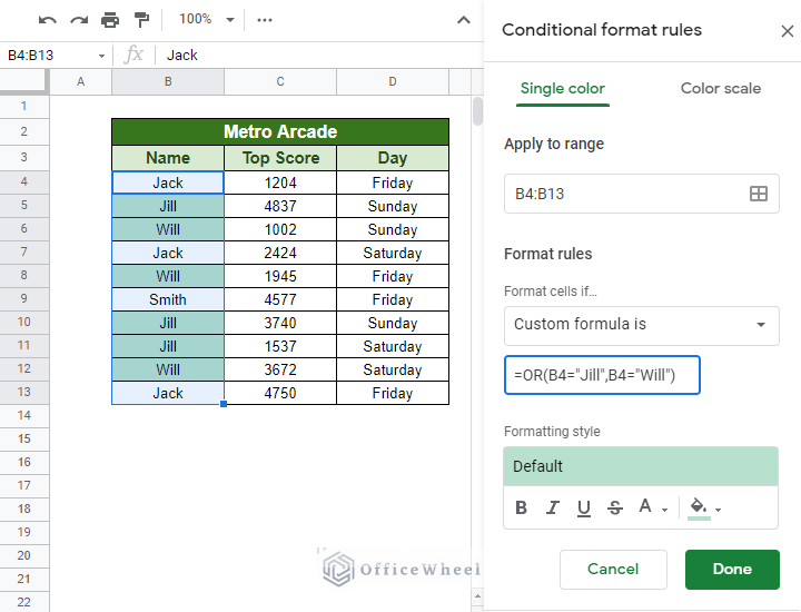
Conditional formatting is a powerful tool in any spreadsheet application. It helps highlight important data in your worksheet no matter how complex the ...

Counting non-blank cells in a spreadsheet is a fairly common affair at every level of the profession. There are many ways to go about it. But today, we will be ...

The COUNTIF function is a fairly basic function in both Excel and Google Sheets. But that doesn’t mean its applications are basic as well. In this article, ...
Hello,
If you want to specify which column’s changes will trigger the timestamp, all you have to do is include an IF ELSE statement inside the existing one. For example, let’s say that the SL column is Column A in the sheet:
if(sheetName == 'Stock'){
    if(range.getColumn() !== 1) return
    else{
      var new_date = new Date();
   spreadSheet.getActiveSheet().getRange(row,4).setValue(new_date).setNumberFormat("MM/dd/yyyy hh:mm:ss");
    }
}
So, if changes are made to any column other than column A or 1, no timestamps will be triggered.
For multiple triggers, we recommend different scripts for each.
I hope it helps!
Hi Max,
I am assuming that you are thinking about extracting the letters ABC from ABC-123. In this case, you can approach it in two ways without even using wildcards.
The first way is to use text functions to extract the number of characters from the string:
=LEFT(B2,LEN(B2)-4)
The LEN(B2)-4 removes the last 4 characters from the string.
For a more dynamic approach, you can look for the hyphen/dash as a delimiter to remove characters before or after it. In this case, to get ABC from ABC-123, the formula will be:
=MID(B2,1,FIND(“-“,B2)-1)
Just replace “-” with any delimiter of your choosing.
However, if you still want to extract using regular expression to get ABC from ABC-123, use this:
=REGEXREPLACE(B2,”[0-9-]”,””)
The regular expression to remove all digits and hyphens is given by [0-9-].
I hope this helps!