Compare Two Columns in Google Sheets (5 Easy Ways)

In this article today, we will be looking at a few ways to compare two columns in Google Sheets.

Most of our methods are an iteration of the base, modified to suit different scenarios and levels of expertise of the user.

Let’s get started.

5 Ways to Compare Two Columns in Google Sheets

1. Basic Side-By-Side Comparison

We start off with a simple side-by-side comparison of rows in two columns. For this, we will be taking advantage of the equals-to (=) operator on the following worksheet.

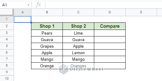
For this example, we will be comparing items from Shop 1 to that of Shop 2. Our result will appear in the Compare column as Boolean.

Our formula is simple:

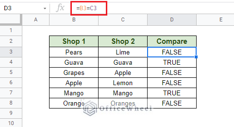
And that’s it!

Now, to bring in some flair to our comparison, we will be adding some extra elements.

Return a Predefined Value (With IF)

Here, we will be using the IF function of Google Sheets to add meaningful messages to our comparison in the Compare column.

Our conditional formula:

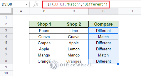
Basically, if the side-by-side values of the two columns match, the formula will return the message “Match”, otherwise, it will show “Different”.

You can put any message to return of your choice.

Note: If you want a case-sensitive comparison the simply replace B3=C3 from the formula with EXACT(B3,C3)

Conditional Formatting the Comparisons

Instead of showing our comparisons in text form, it can be a better idea to highlight the matches in color, for better representation of matched data. Thankfully, Google Sheets allows us to do just that with its conditional formatting option.

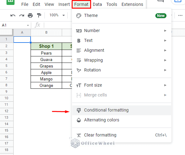
To open the conditional formatting menu, simply navigate to the Format tab at the top of the window. Here, select the Conditional formatting option.

This should open the Conditional format rules menu tray. Then follow these steps:

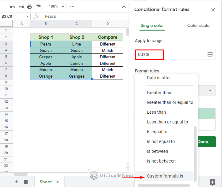
Step 1: Select the range of cells that you want to apply your formatting to. We have chosen B3:C8.

Step 2: Select the Custom formula is option from the Formula rules drop-down menu, as seen in the following image.

Step 3: Enter the formula: =$B3=$C3

Note: Locking the columns with absolutes ($) helps to format the entire row.

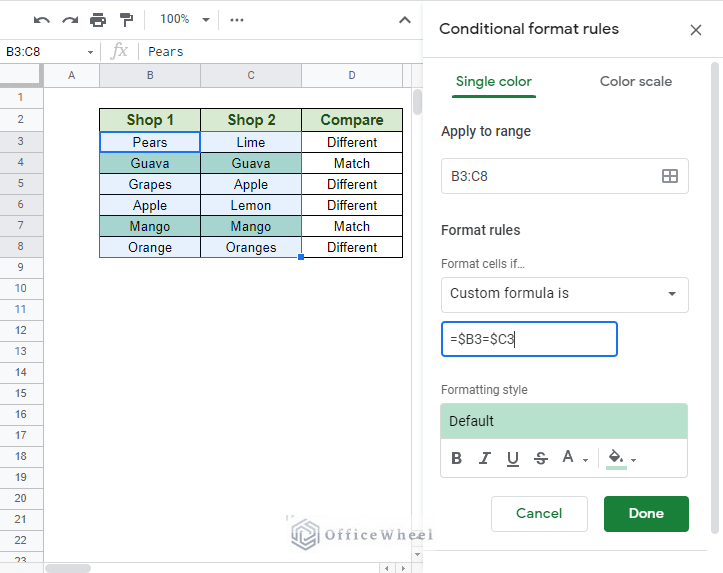
Step 4: Apply the desired formatting and click Done.

So far, we have discussed the absolute fundamental way to compare two columns in Google Sheets. Moving forward, we will see how to apply functions and formulas to make our comparisons more intuitive and suited to various scenarios.

2. Full Column Range Comparison in Google Sheets

In this section, we will be doing a comparison of the whole column, not just the rows/cells side-by-side. For this, we have to get creative and use some functions of Google Sheets.

I. Using the COUNTIF function

The first function we will be using is COUNTIF.

Fundamentally, the COUNTIF function will count the number of occurrences of our comparison condition (from the Shop 2 column) in the designated column (Shop 1).

To that end, our formula is:

Note: We have locked our range (press F4 once) to stop it from moving as we apply the formula down the Compare column.

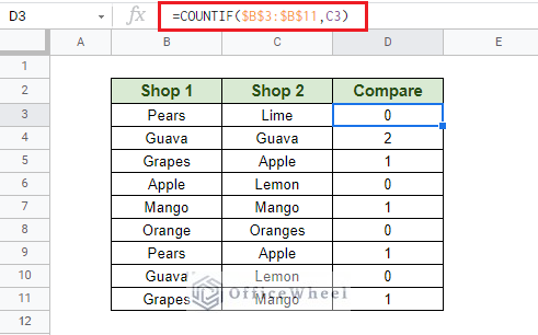
As you can see, the Compare column now shows the number of occurrences of each item in Shop 2 in Shop 1.

But what we wanted is simply whether the items in Shop 2 are also present in Shop 1. To bring up that comparison we have to add a condition that gives us a Boolean value: True, if the count is more than 0.

Our new formula:

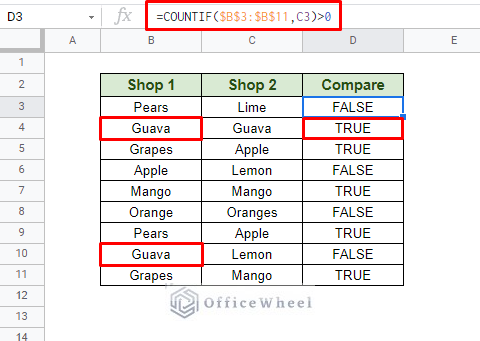
We have just successfully compared the entire range of two separate columns.

II. ARRAYFORMULA

Now we are going to look at an iteration of the previous formula that not only compares the two columns but also handles exceptions and errors.

For our comparison condition, we will use a combination of IF and MATCH functions. our formula:

Note: Since we are comparing Shop 2 against Shop 1, the range of Shop 2 will come first, C3:C11.

To handle errors, we will implement the IFERROR function.

Finally, the range output this time will be in array form, thus we have to use the ARRAYFORMULA function. The advantage of using arrays is that only need to apply this formula to the first cell of the column, and it will automatically populate with values.

The final form of our formula:

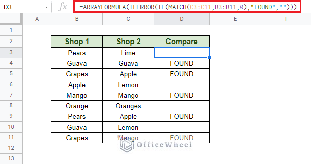
3. Conditional Comparison of Columns in Google Sheets

This section should be simpler than most as it takes from the IF conditional function discussed in method 1.

This time, we have a worksheet like this.

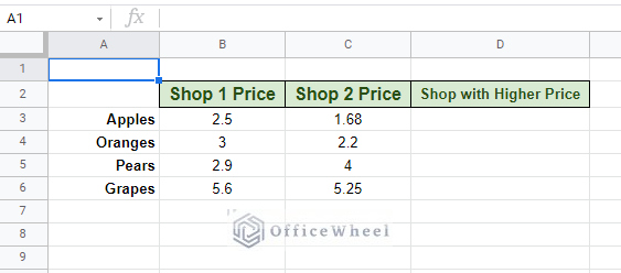
As you may have already guessed, we will be comparing the prices of the two columns, Shop 1 Price and Shop 2 Price, and output the shop with the higher price of products.

Our formula at D3 is pretty simple:

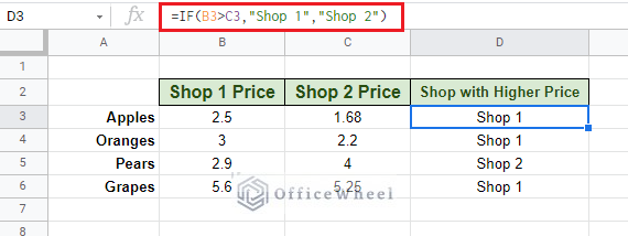
Extra: Find Maximum/Minimum of Two Columns

As a small sendoff for this section, let us show you how you can extract the maximum or minimum prices among the two columns.

For Maximum:

For Minimum:

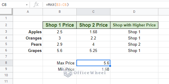
4. Compare and Search for Missing Data

This comparison method stems from the first process discussed in method 2, the COUNTIF function.

It is fairly simple, even similar to some of the methods discussed previously. But again, the only added modification comes in the form of the IF function. We will be simplifying our array formula with MATCH (method 2, part 2) to achieve a similar result.

Our formula:

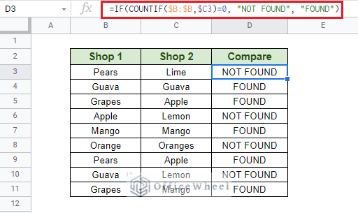
Using FILTER Function to Compare and Extract Missing Values

So far, we have found that values are missing, but what if we want to extract these missing values?

The FILTER function makes our life that much easier in such a case.

The syntax:

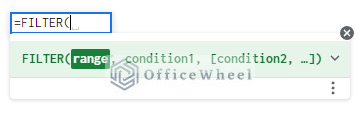
Our objective is to extract all the values from column Shop 1 that are missing in Shop 2. Our formula:

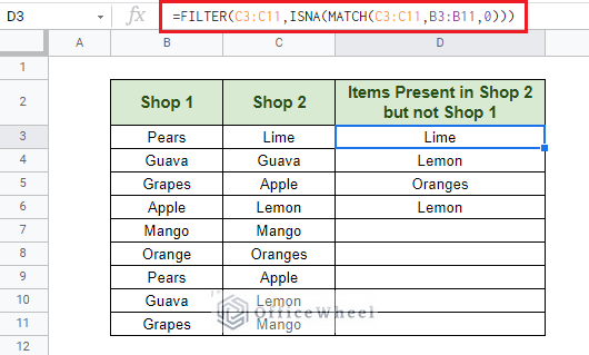
Note that Oranges is considered missing from Shop 1 since Shop 1 contains the word “Orange” not “Oranges”. It has to be a perfect match.

5. Compare and Make a List of Matches from Two Columns

In our last method, we have extracted the missing components when comparing two columns. This time, we will be doing just the opposite by making a list of all the matches after comparing the two columns.

We will use the VLOOKUP function to determine whether the value of one column (Shop 1) exists in another (Shop 2).

The syntax:

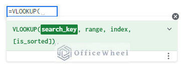
In cell D3 we enter the formula:

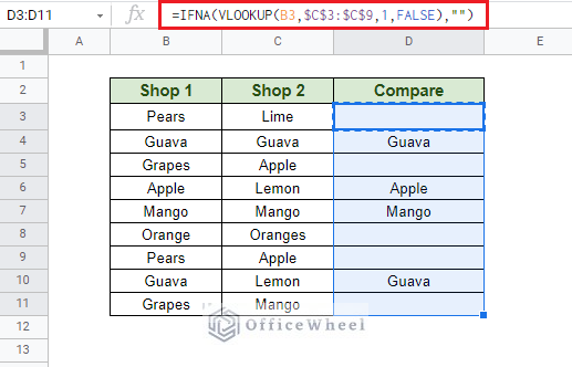
Note: We are using the IFNA function to catch the #NA error and return a blank.

An alternative to using VLOOKUP would be using the classic combination of INDEX and MATCH functions.

The formula goes like:

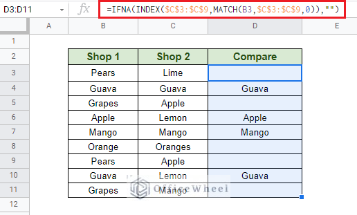
Final Words

We hope that all the methods and scenarios we have discussed in regard to comparing two columns in Google Sheets will help you in your work.

Please feel free to leave us any queries or advice you might have for us in the comments below.