How to Copy and Paste Conditional Formatting in Google Sheets

In this article, we will discuss thoroughly how to copy and paste the conditional formatting in Google Sheets. You can then apply the learnings in your day-to-day life as well as in your work life.

Table of Contents

A Sample of Practice Spreadsheet

Copy Paste Conditional Formatting

4 Methods to Copy And Paste Conditional Formatting in Google Sheets

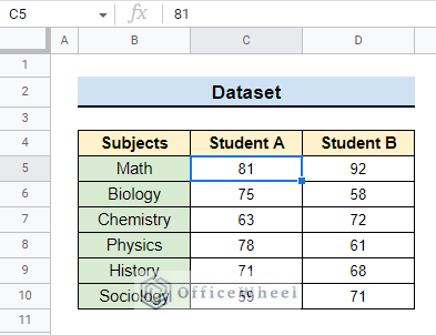
We have a dataset with the marks of two students in different subjects. The marks less than 65 obtained by Student A in all subjects with conditional formatting are highlighted. We will try to copy and paste the same conditional formatting for Student B.

1. Using the Paint Format Tool

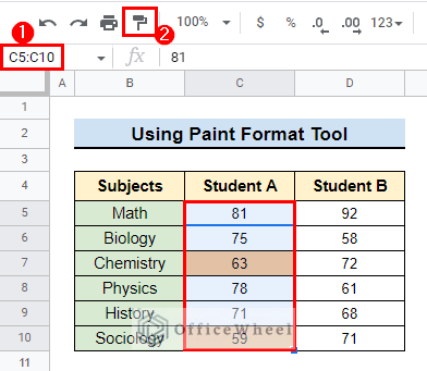
The easiest way to copy and paste Conditional Formatting is the Paint format tool. You may already have seen or used this tool in your Google Sheets. Did you know that it can effortlessly copy and paste conditional formatting too? Let’s see how it is done:

First, select the column or cells which contain the conditional formatting and click on the Paint format tool from the Toolbar. We select column C5:C10.

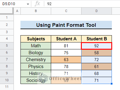
After that, click on the first cell of the column where you want to paste the formatting. In our example, we click on cell D5 to activate it. You can see that conditional formatting is already copied without much hassle.

You can apply this method to any single cell too.

Copy and Paste from Another Sheet Using Paint Format

You can even copy-paste conditional formatting from another sheet too using Paint format. Just follow these steps:

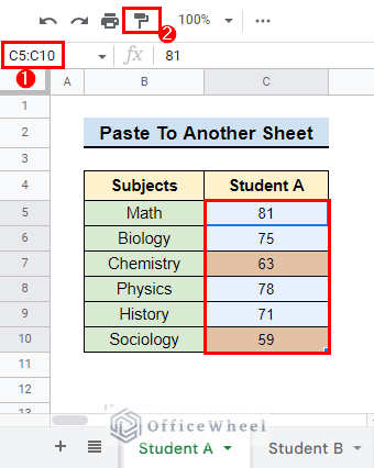
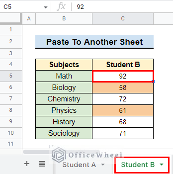
For this, let’s consider the marks of Student A and Student B are in two separate sheets. We will copy the formatting applied to the marks of Student A and paste the similar formatting to Student B which is on another sheet.

First, select the column or cells which contain the conditional formatting and click on the Paint format tool from the Toolbar.

After that, click on the cell or select the range of cells in another sheet where you want to paste the formatting. In our example, we click on cell C5 of the Student B worksheet.
You will see that your conditional formatting is copied.

2. Utilizing Paste Special Feature

The Paste Special feature is a handy tool for copying and pasting conditional formatting in Google Sheets. It is easier than you can imagine. Just follow these steps:

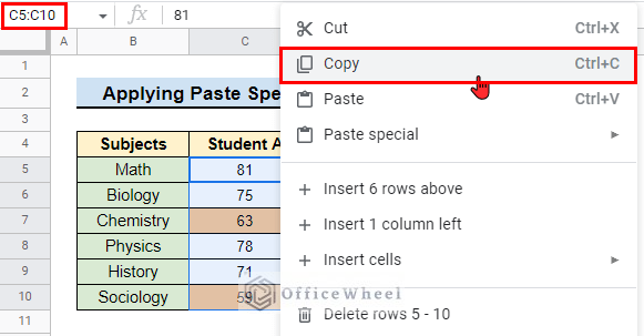
First, copy the column from where the conditional formatting is by using CTRL+C or from the dialogue box after right-clicking on the mouse. We Select column C5:C10 and copy it.

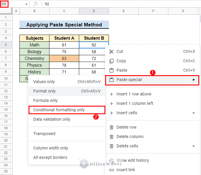
Then, select the entire column or the first cell of the column where you want to paste the conditional formatting and right click on the mouse, and go to Paste special > conditional formatting only. We select cell D5 in our dataset example.

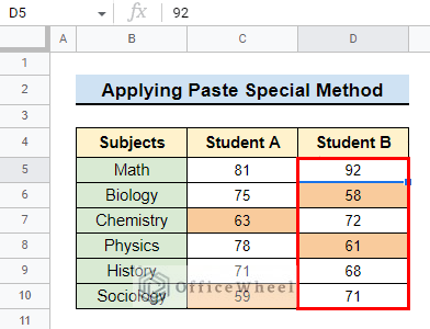
Finally, you will see that the conditional formatting has been copied to the desired column.

Similar Readings

3. Duplicating the Applied Rule

Another way of copy-pasting conditional formatting in Google Sheets is to duplicate the formatting rule.

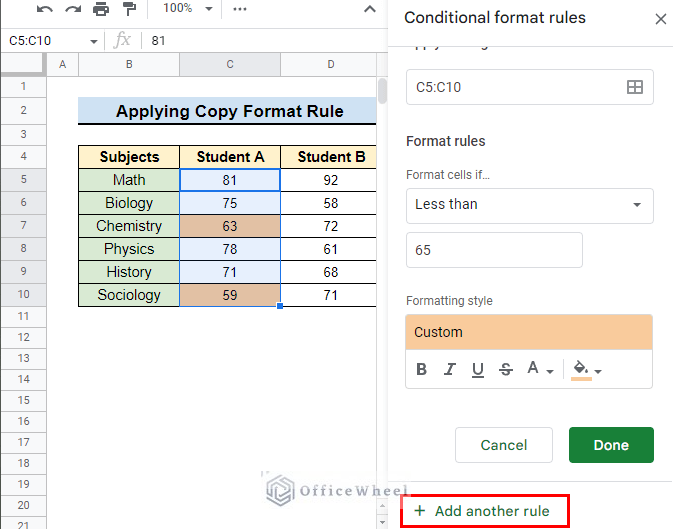
First, open the conditional format rules sidebar and select the existing rule and click on Add another rule from the bottom of the sidebar.

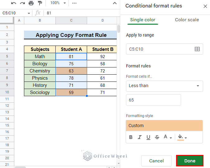
Next, press Done.

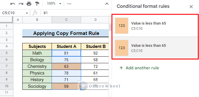
Now, you will see two identical rules on the side panel.

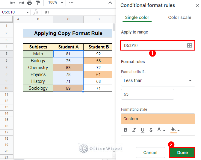
Next, open the duplicate or the second rule that you have just created and update it to your desired range. We type D5:D10 as this is where we want to paste the conditional formatting.
Finally, press Done and you have two identical conditional formatting rules for two different columns.

4. Expanding the Range

Conditional formatting can be copy-pasted by expanding the existing range too. Just follow these steps:

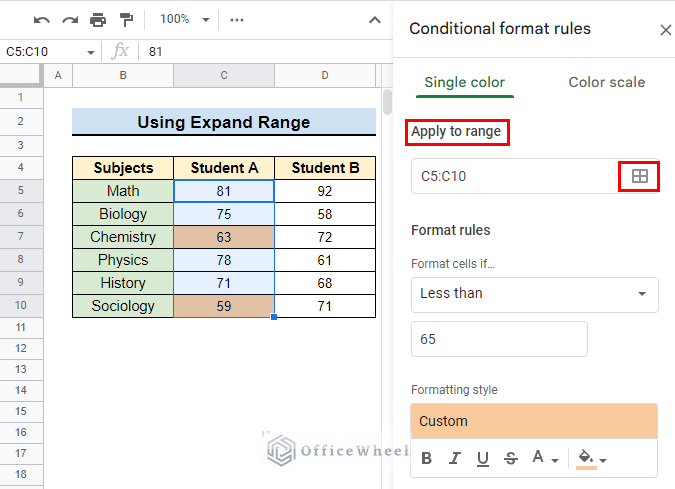
First, select the existing rule from the conditional formatting rules sidebar and click on the Select data range icon in the Apply to range panel.

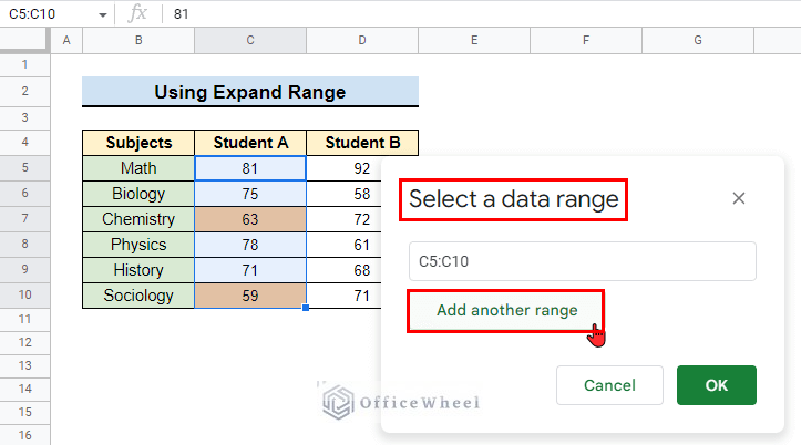
Now, press Add another range from the popup that appears and select your desired range.

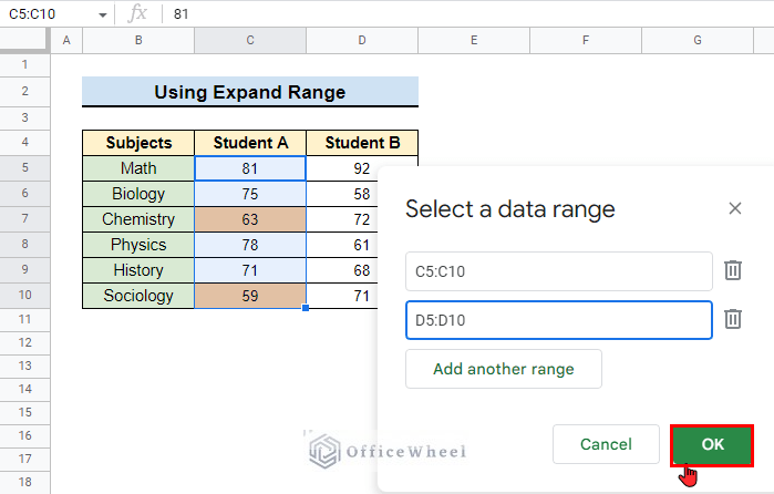
For our example, we type D5:D10.
Next, press OK to have your conditional formatting copied to the new range.

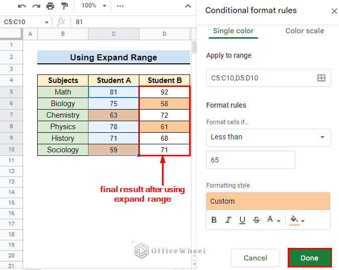
Finally, press Done and you have your new dataset.

Conclusion

Being able to copy and paste the conditional formatting in Google Sheets is a great technique to possess. It can come in handy to you anytime while working in Google Sheets. In this article, we showed you how to copy and paste the conditional formatting in Google Sheets in 4 methods.

We hope this article was helpful to you and that you found the methods easy.

Also, check out other articles on OfficeWheel that may help you to improve your Google Sheets work knowledge.