Google Sheets Pivot Table: How to Remove Grand Total or Subtotal

In this simple tutorial, we will show you why and how to remove the Grand Total field of a Google Sheets pivot table.

Let’s get started.

Table of Contents

Why do we need to remove the Grand Total Row or Column from a Pivot Table?

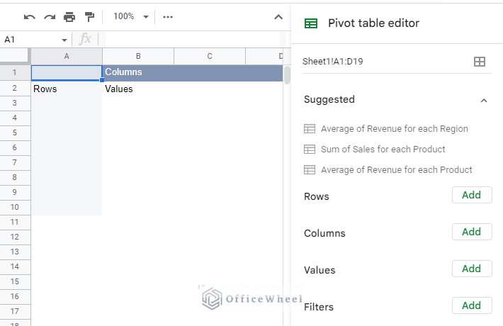
When we create a pivot table in Google Sheets, we get this empty canvas by default:

We can populate this with rows, columns, and other values that will help us summarize large quantities of data. This is the primary function of a pivot table.

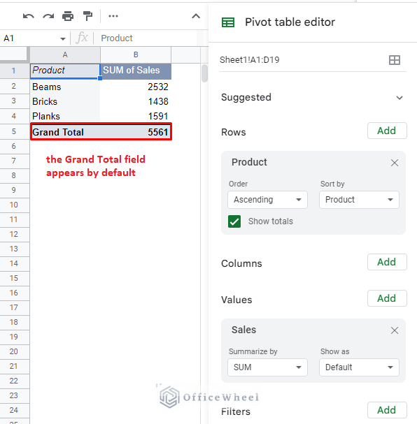
As you can see, when we add a row and populate the table with values, a Grand Total row appears by default. A Grand Total column would’ve also appeared if we added a column condition to the pivot table.

While this Grand Total field does give us useful information, it may not always be required. There are even instances where the Grand Total field might prove to hamper the data analysis itself.

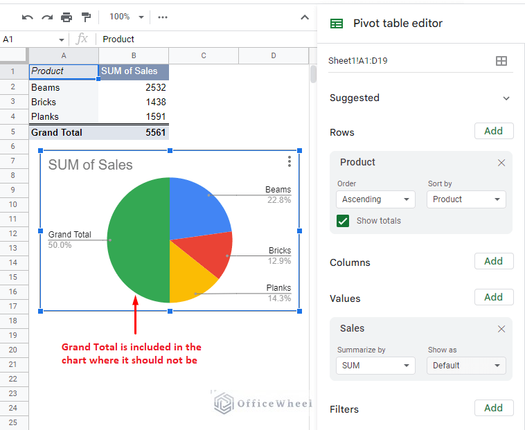
For example, let’s say we insert a chart representing the Sum of Sales for each type of Product.

Insert > Chart

What we get is something like this:

We get a chart that includes the Grand Total field when it should not be there!

It takes up 50% of the data and does not give a true summary of the source dataset.

Getting the intrusive Grand Total field included in the data chart is the primary reason why users want to remove the Grand Total field from the pivot table.

Let’s see how it’s done.

How to Remove the Grand Total from a Google Sheets Pivot Table

Remove Grand Total from Row

In our current pivot table, we added a row that automatically included the Grand Total column. We will be working with this first.

If you come from Excel, you might already know that to remove this Grand Total or Subtotal field, you have to do so from the Design tab. But Google Sheets makes things much simpler by allowing us to format the entirety of the pivot table right from the Pivot Table Editor.

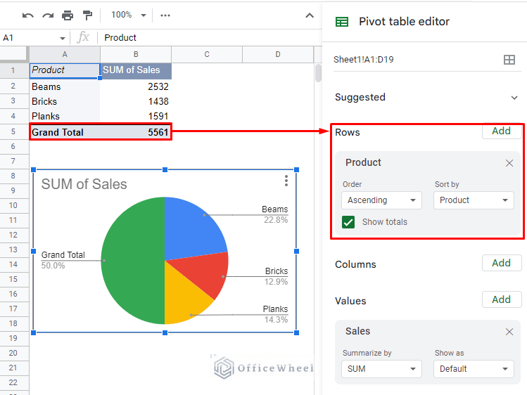
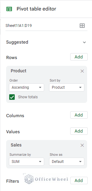
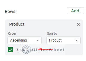
When you add any row to the pivot table, a row panel will appear where you can customize how the row data will be presented. Here, a small checkbox will also appear at the bottom of the panel called ‘Show totals’. This remains checked by default.

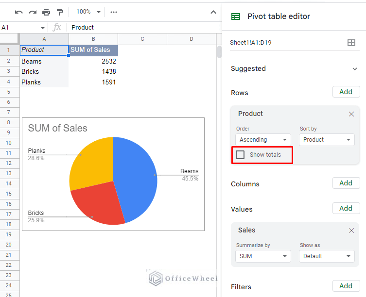
This checkbox is the option that shows the Grand Total in the pivot table. Unchecking this option will remove the Grand Total from the row of a Google Sheets pivot table.

Unchecking the ‘Show totals’ option immediately removes the Grand Total row and the Grand Total option from the chart.

Remove Grand Total from Column

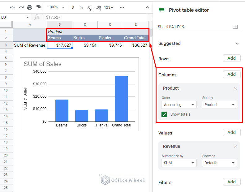
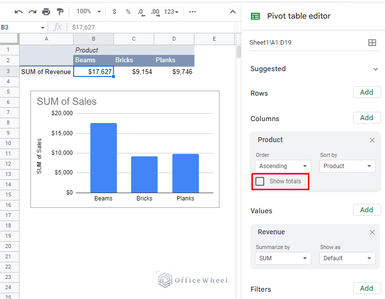
Now let’s look at another orientation of the pivot table. Here, the table layout and values are dependent on the columns and shows the sum of Revenues for each Product.

Like before, a field of Grand Total is included in the table. This time, it is as a column.

And also, like before, the Grand Total is taking up space in the following chart and disrupting the summarization of the data in Google Sheets.

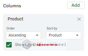
Like rows, adding a new column field to a Google Sheets pivot table automatically comes with the ‘Show totals’ checkbox checked. This makes the Grand Total field appear by default.

With Google Sheets providing us with the easy-to-use Pivot table editor, similar problems will have similar solutions.

To remove the Grand Total field from the column of a Google Sheets Pivot table, simply uncheck the ‘Show totals’ checkbox.

Alternative Approaches to Remove Grand Total from a Google Sheets Pivot Table

It may be also possible that you do not want to completely remove the Grand Total field from the pivot table, but only from the Chart created from it.

In that case, we have two alternative processes to remove the Grand Total field from a Google Sheets Pivot table:

Hide the Row or Column
Change the Data Range of the Chart

1. Hide the Row or Column from the Worksheet that contains Grand Total

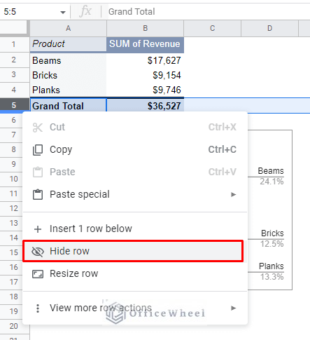
We can simply hide the entire row or column that contains the Grand Total field in the pivot table.

Step 1: Right-click on the Row number or Column number of the worksheet to bring out the options.

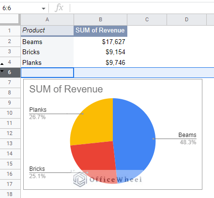
Step 2: Click on the Hide row (or Hide column) option to remove the Grand Total from the Chart.

As you can see, the Grand Total is still there, only hidden from the calculation.

2. Change the Data Range of the Chart

The other, and frankly much better, alternative to remove the Grand Total from a pivot table chart is to change the data range.

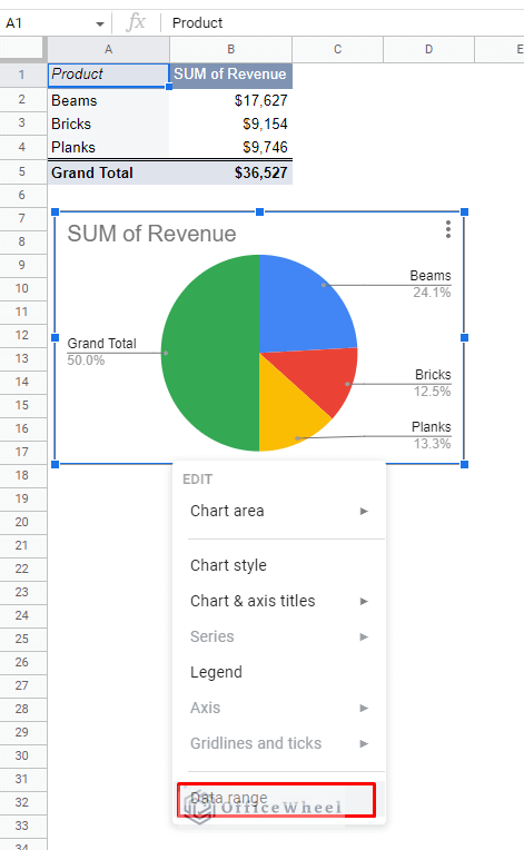
Step 1: Right-click over the chart to bring out the options. Click on the Data range option to open the Chart editor panel.

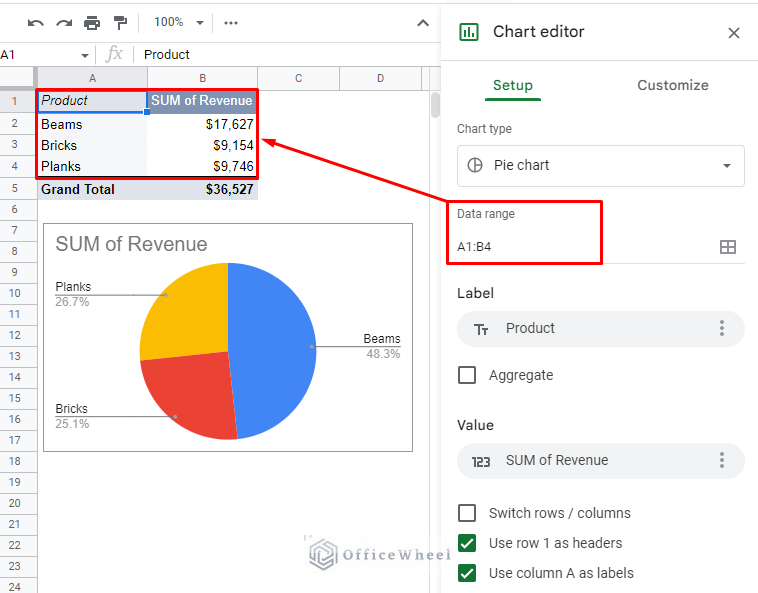
Step 2: Update the Data range of the chart in the editor to exclude the row or column that contains the Grand Total. We have updated our data range from A1:B5 to A1:B4.

The Grand Total no longer falls in the range of the chart and is thus removed from it.

Final Words

That concludes the ways we can remove the Grand Total field of a Google Sheets pivot table. The Pivot table editor allows us to simply turn off the ‘Show totals’ option to remove the field entirely. While hiding and changing the data range of the chart created using the pivot table works well as well.

Feel free to leave any queries or advice you might have in the comments section below.