The SEARCH function is a very popular function in Google Sheets. We can use this function to determine the position of a character or to find a substring within a string. This function helps Google Sheets users in numerous ways. In large datasheets, it helps to search for relevant data very quickly. In this article, we will describe the anatomy of the SEARCH function and represent its various uses in Google Sheets.
A Sample of Practice Spreadsheet
You can download the practice spreadsheet from the download button below.
What Is SEARCH Function in Google Sheets?
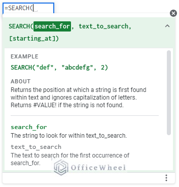
The SEARCH function returns the position of a character first found in a text string. It is case-insensitive, so it can not differentiate between upper-case and lower-case capital letters.
Syntax
The Syntax of the SEARCH function is shown below.
Arguments
| ARGUMENT | REQUIREMENT | Function |
|---|---|---|
| search_for | Required | The character that is searched for in the string. It can be a character, substring, or array of strings. |
| text_to_search | Required | Here, the function searches for the first presence of the “search_for” string. |
| [starting_at] | Optional | This number guides the function from where the search starts. If you don’t put any number, it will take 1 as default and start searching from the beginning. |
Output
The formula SEARCH(“a”, “Football is a popular game.”,1) will return 6 because the first “a” in the string “Football is a popular game.” is in the 6th position from the beginning.
5 Suitable Examples of Using SEARCH Function in Google Sheets
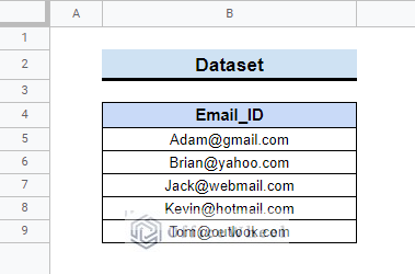
Suppose, we have a dataset containing some email ids. The email ids contain the first name of the users and then the email domain names separated by “@”. We will use this dataset to show some uses of the SEARCH function.
1. Find Position of Character
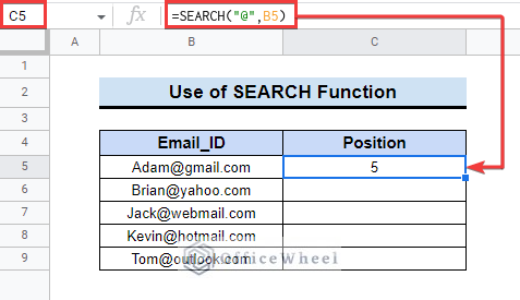
The SEARCH function helps to know the position of a character in a string. If the character is repeated multiple times, it will show the 1st position of the character. Here you can use the SEARCH function to find the position of a character. Follow the steps to learn how to do that.
📌 Steps:
- First, select cell C5 and insert the following formula in the formula bar.
=SEARCH("@",B5)- Then, this will return the position of the “@” symbol in the string.
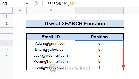
- Finally, drag down the fill handle tool to apply the formula up to cell C9.
Read More: How to Search in All Sheets in Google Sheets (An Easy Guide)
2. Extract Names from Email ID
You can use the SEARCH function to extract the user names of the email ids. You need to combine the LEFT function with the SEARCH function to do that. The LEFT function returns the text from the beginning or the left side of a string. Follow the steps below to extract the user names.
📌 Steps:
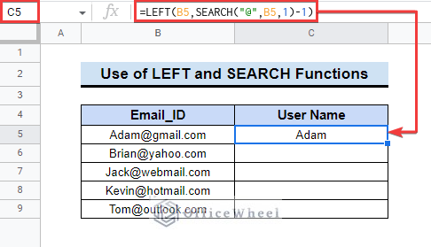
- First, to extract the user names of the email ids, enter the below formula in cell C5.
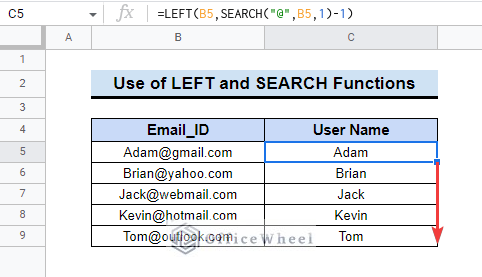
=LEFT(B5,SEARCH("@",B5,1)-1)- Next, copy the formula to other cells of the table, or simply drag it down or double-click on the fill handle tool.
- After that, you will see the formula result in C5:C9.
Formula Breakdown:
- SEARCH(“@”B5,1): It searches for “@” in the B5 string from the 1st character.
- LEFT(B5,SEARCH(“@”,B5,1)-1): This will extract the string just before the “@” symbol from the beginning.
Read More: How to Create a Search Box in Google Sheets (4 Easy Methods)
3. Remove Characters from Left
You can remove characters from the start of a string using the RIGHT, LEN, and SEARCH functions. The RIGHT function returns the substring from the right side or end of a string. The LEN function returns the length/total characters number of the string. Here, the SEARCH function will find a character and keep the right substring up to that character. The steps to do that are mentioned below.
📌 Steps:
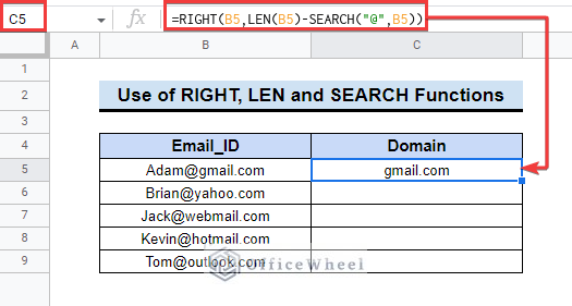
- First, insert the following formula in cell C5.
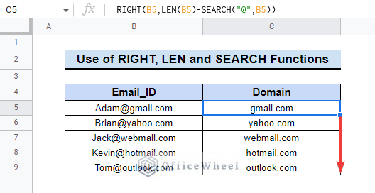
=RIGHT(B5,LEN(B5)-SEARCH("@",B5))- Next, copy the formula to other cells using the double-click or drag-down feature of the fill handle tool. This way you will get only the domain names as output.
Formula Breakdown:
- SEARCH(“@”,B5): This function locates the position of the “@” symbol.
- LEN(B5)-SEARCH(“@”,B5): This formula is the difference between the total string length and position of “@”. Which is (14-5)=9 for cell C5.
- RIGHT(B5,LEN(B5)-SEARCH(“@”,B5)): This formula returns the 9 characters starting from the right side or end of the string.
Read More: How to Remove First Character in Google Sheets
4. Search for Substring
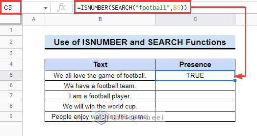
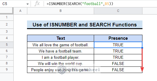
If you want to be confirmed about the presence of any word or substring in a dataset, you can use the ISNUMBER and SEARCH functions together. The ISNUMBER number function checks if a value is present or absent in a string. If the value(here substring) is present then it will return true otherwise false. Follow the steps below to do it by yourself.
📌 Steps:
- Now, to search for the presence of a substring, enter the below-mentioned formula in cell C5.
=ISNUMBER(SEARCH("football",B5))- After that, drag down the fill handle tool to copy the formula.
Formula Breakdown:
- SEARCH(“football”,B5): This formula looks for “football” in the text string.
- ISNUMBER(SEARCH(“football”,B5)): This formula shows the result as “TRUE” or “FALSE” according to the presence of the mentioned substring.
Read More: How to Search in a Column in Google Sheets (3 Suitable Ways)
5. Find and Replace Text
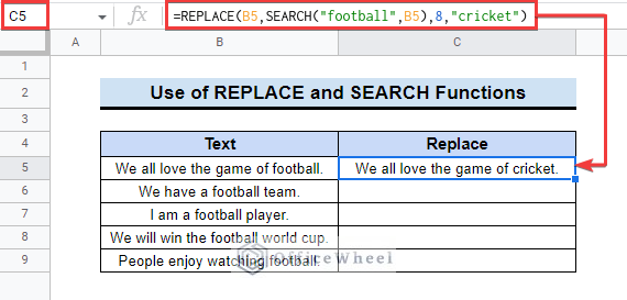
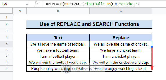
You can easily use the SEARCH function to replace a text in a string with the help of the REPLACE function. The SEARCH function will find the text and the REPLACE function will replace it with a given alternative text.
📌 Steps:
- First, insert the following formula in cell C5.
=REPLACE(B5,SEARCH("football",B5),8,"cricket")- Next, to replace “football” with “cricket” in all the texts, drag down the fill handle tool.
Formula Breakdown:
- SEARCH(“football”,B5): This formula finds “football” in B5.
- REPLACE(B5,SEARCH(“football”,B5),8,”cricket”): Here, after the SEARCH function, 8 means the total character number of the substring, and “cricket” is the new substring which will replace the previous substring.
Read More: How to Search and Replace in Google Sheets (2 Easy Ways)
Alternative to SEARCH Function in Google Sheets
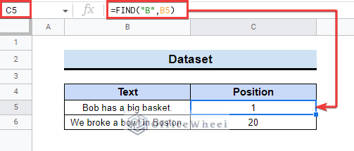
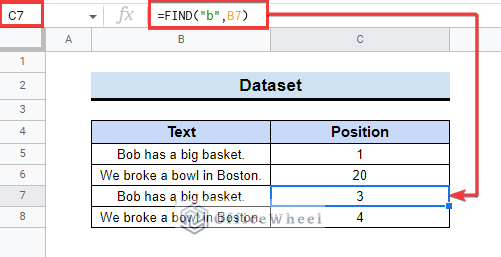
There is an alternative to the SEARCH function in Google Sheets. That is the FIND function. The SEARCH function and the FIND function are pretty much the same. But the main difference between them is that the FIND function is case-sensitive, and the SEARCH function is not. So, if you need to find any case-sensitive character then you need to apply the FIND function, not the SEARCH function.
- In the following example, you can see, for capital “B” the FIND function will show a position. The first formula in C5 is given below.
=FIND(“B”,B5)- But, for small “b” it will show another position as the FIND function is case-sensitive. You can check it by entering the following formula in C7.
=FIND(“b”,B5)This is the advantage of using the FIND function.
Read More: How to Search for Text in Range in Google Sheets (4 Simple Ways)
Things to Remember
- The SEARCH function returns the position of a character. However, if the character is present more than once in a string, then it will only return the first occurrence.
- The SEARCH function returns a #VALUE! error when it is unable to find anything in the string.
Conclusion
We have shown you the uses of the SEARCH function in Google Sheets. Hopefully, the examples above will be enough for you to understand the applications of the SEARCH function. Please use the comment section below for further queries or suggestions. You may also visit our OfficeWheel blog to explore more about Google Sheets.
Related Articles
- Remove Characters from a String in Google Sheets (6 Easy Examples)
- How to Remove Text after Character in Google Sheets (5 Methods)
- Convert Text to Date in Google Sheets (3 Easy Ways)
- How to Remove Everything after Character in Google Sheets
- How to Format Date with Formula in Google Sheets (3 Easy Ways)
- Remove Everything after Character Using Google Sheets Formula

