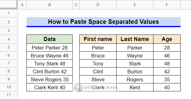
We often append various related values in a cell by putting a delimiter in between the values. But how can we paste or split these appended data into different cells? In this article, we’ll demonstrate 2 easy ways to paste space separated values in Google Sheets. Also, we’ll discuss how we can split space separated values instead of using paste. The following image is an overview of the result we require.
A Sample of Practice Spreadsheet
You can copy our practice spreadsheets by clicking on the following link. The spreadsheet contains an overview of the datasheet and an outline of the discussed ways to paste space separated values in Google Sheets.
2 Easy Ways to Paste Space Separated Values in Google Sheets
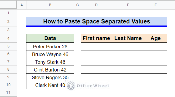
First, let’s get familiar with our dataset. The dataset contains a list of first names, last names, and ages appended and separated by spaces. We want to paste these space separated values to separate columns. Now let’s get started.
1. Using Clipboard Menu
We can apply Split Text to Columns command from the clipboard menu options. The clipboard menu is generated while applying the Paste command. And then the Split Text to Columns command can put the space separated values into different columns.
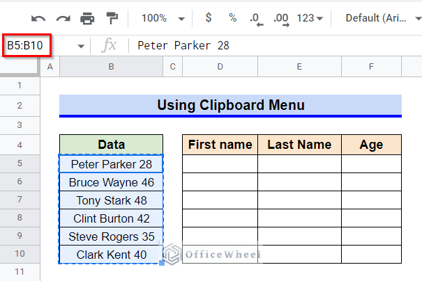
Steps:
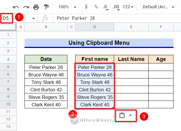
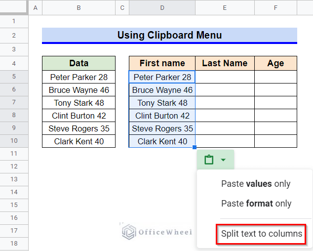
- Afterward, select Cell D5 and paste the range using the keyboard shortcut CTRL+V. At this point, the clipboard for paste formatting will be visible. Click on the Clipboard menu.
- From the appeared options, select the Split Text to Columns command.
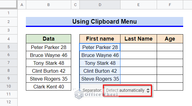
- At this time, a new clipboard will appear, where you can select the separator to execute the Split Text to Columns Click on the Separator clipboard.
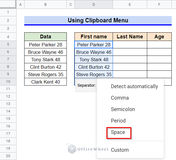
- A list of separators will be visible now. We’ll select the Space option from here. You can choose the separator you require. You can also insert a custom separator if it isn’t available in the appeared list.
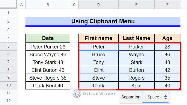
- As soon as you select the Space option as the separator for the Split Text to Columns command, the copied values will be split into required columns.
Read More: [Solved!] Paste Values Is Not Working in Google Sheets (2 Fixes)
2. Applying Split Text to Columns Command
Instead of using the clipboard, we can perform the Split Text to Columns command from the Data ribbon. Keep reading to learn how.
Steps:
- Follow the first two steps of the previous method to copy and paste the range B5:B10 to D5:D10 by using the Ctrl+C and Ctrl+V keyboard shortcuts.
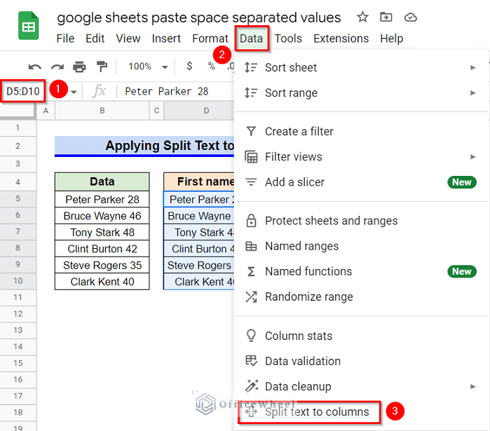
- Now, select the range D5:D10 and go to the Data ribbon.
- Select the Split Text to Columns command.
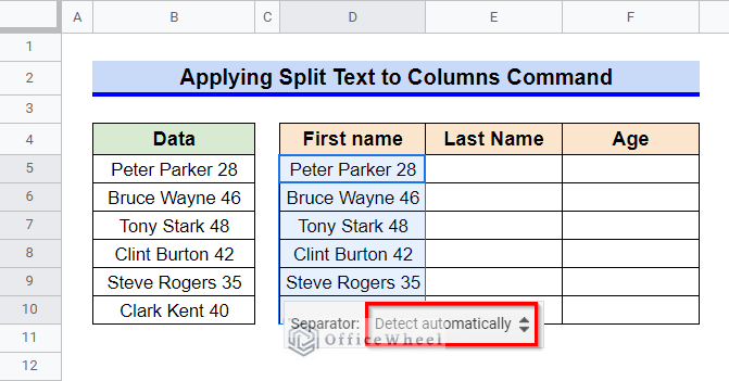
- A clipboard will appear at this time, where you can select the separator to execute the Split Text to Columns command.
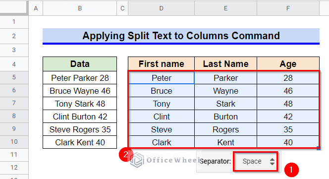
- A list of separators will be visible when you click on the Separator We’ll select the Space option from there. This will provide us with the required result like the following.
Alternatives to Paste Space Separated Values in Google Sheet
Instead of using the Split Text to Columns command to paste space or any other delimiter separated values we can use the SPLIT function to allocate them in adjacent columns. One of the limitations of using the Split Text to Columns command is that it can’t separate strings that contain multiple delimiters at a time. Whereas, we can combine the SPLIT and REGEXREPLACE functions to perform such operations. We’ll discuss this in the next section. Now, let’s get started with learning the execution of the SPLIT function.
1. Employing SPLIT Function
The SPLIT function is an exclusive function in Google Sheets. It can cleave strings around a specified delimiter or character and puts each snippet into cells of adjacent columns.
Steps:
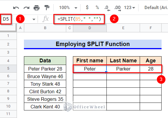
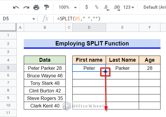
- Firstly, activate Cell D5 by double-clicking on it.
- Then, type in the following formula-
=SPLIT(B5," ","")- Afterward, press the Enter key to get the required output.
- Now, select Cell D5 again and then hover the mouse pointer above the bottom-right corner of the selected cell.
- The Fill Handle icon will be visible at this time.
- Finally, use the Fill Handle icon to copy the formula to other cells of Column D.
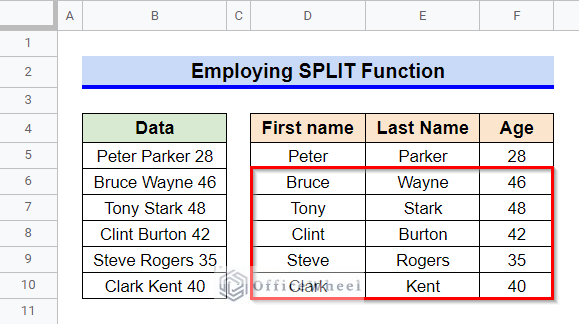
- The final output looks like the following after using the Fill Handle tool.
2. Joining ARRAYFORMULA and SPLIT Functions
We can join the ARRAYFORMULA function with the SPLIT function to get the same result as the previous method without using the Fill Handle tool. The SPLIT function is a non-array function. Hence, we require joining the ARRAYFORMULA function with it if we want the SPLIT function to deal with an array.
Steps:
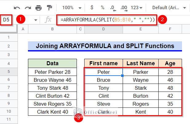
- Activate Cell D5 by selecting it first and then using the function key F2.
- Afterward, insert the following formula-
=ARRAYFORMULA(SPLIT(B5:B10," ",""))- Finally, get the required output by pressing Enter key. And as you can see, we have performed the splitting text operation without using the Fill Handle tool.
Formula Breakdown
- SPLIT(B5:B10,” “,””)
The SPLIT function divides the texts in each cell of range B5:B10 into separate cells of adjacent columns around the space (“ ”) delimiter.
- ARRAYFORMULA(SPLIT(B5:B10,” “,””))
The ARRAYFORMULA function helps the non-array function SPLIT to deal with and display an array.
3. Combining INDEX and SPLIT Functions
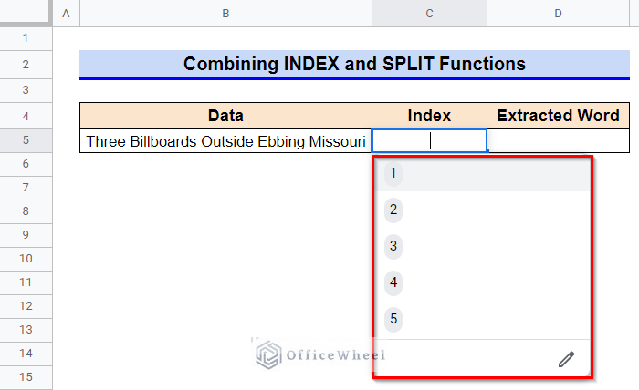
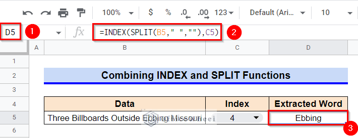
Sometimes, we may require only a specific part of a string. Instead of splitting the entire text, we can simply extract the required part by combining the SPLIT and INDEX functions. We’ll use the following dataset for this operation where we’ll extract a specific space separated word from the data based on an index from a drop-down list.
Steps:
- To start, click on the drop-down icon of the Index column.
- At this point, a list of index options will appear. Select the index you require.
- Now, select Cell D5 and type in the following formula-
=INDEX(SPLIT(B5," ",""),C5)- Finally, press Enter key to get the required result.
Formula Breakdown
- SPLIT(B5,” “,””)
First, the SPLIT function returns a range by dividing each space separated value into different cells.
- INDEX(SPLIT(B5,” “,””),C5)
Later, the INDEX function returns the content of the cell in the range specified by the SPLIT function based on the offset index provided in Cell C5.
- Now, if you change the index, the extracted word changes automatically.
How to Paste Multiple Delimiter Separated Values in Google Sheets
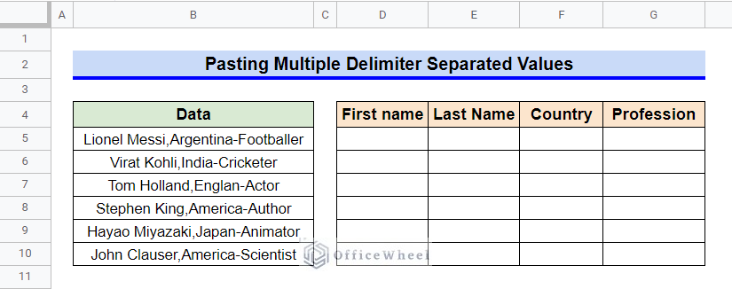
As we said previously, we can combine the SPLIT and REGEXREPLACE functions to paste or split texts around multiple multiple delimiters. We’ll use the following dataset for this example. The dataset contains a list of first names, last names, origin countries, and professions for a list of people separated by a space (“ ”), a comma (“,”), and a hyphen (“-”) delimiter. Now, let’s perform the splitting operation.
Steps:
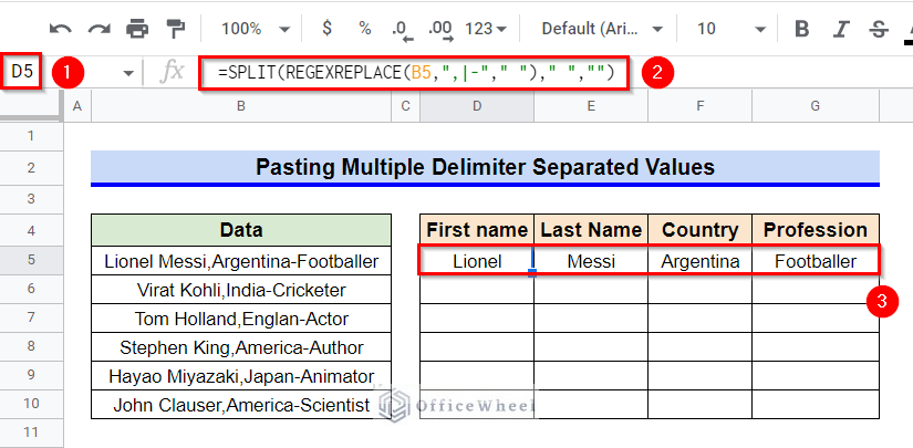
- Firstly, select Cell D5.
- Afterward, insert the following formula-
=SPLIT(REGEXREPLACE(B5,",|-"," ")," ","")- Later, get the required output by pressing the Enter key.
Formula Breakdown
- REGEXREPLACE(B5,”,|-“,” “)
The SPLIT function can’t actually divide texts based on multiple delimiters. Hence, the REGEXREPLACE function is used for substituting every other output to a single delimiter. Here, we have substituted every other delimiter with spaces (“ ”).
- SPLIT(REGEXREPLACE(B5,”,|-“,” “),” “,””)
And now, the SPLIT function divides the space separated values into adjacent cells of a row.
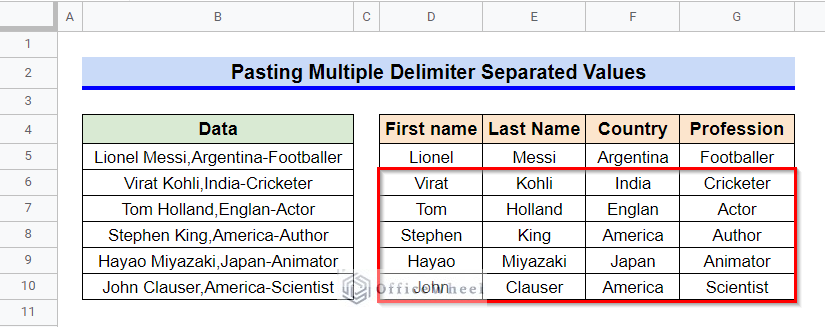
- Finally, use the Fill Handle icon to copy the formula to other cells.
Read More: How to Paste Values Only in Google Sheets (4 Quick Ways)
Conclusion
This concludes our article to learn how to paste space separated values in Google Sheets. However, you can use the same methods for other delimiter separated values too. I hope the demonstrated methods were ideal for your requirements. Feel free to leave your thoughts on the article in the comment box. Visit our website OfficeWheel.com for more helpful articles.

