We often use the COUNTIF function for counting the number of cells based on a specific criterion. However, when we use text criteria in the COUNTIF function, it usually isn’t case-sensitive. Hence, if we require a case-sensitive COUNTIF operation, we can’t achieve the desired output with the COUNTIF function. In this article, I’ll discuss 7 easy ways to execute a case sensitive COUNTIF operation in Google Sheets.
A Sample of Practice Spreadsheet
You can copy our practice spreadsheets by clicking on the following link. The spreadsheet contains an overview of the datasheet and an outline of the discussed examples of how to execute a case sensitive COUNTIF operation in Google Sheets.
6 Easy Ways to Execute Case Sensitive COUNTIF in Google Sheets
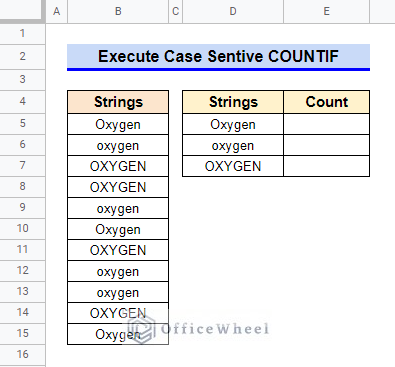
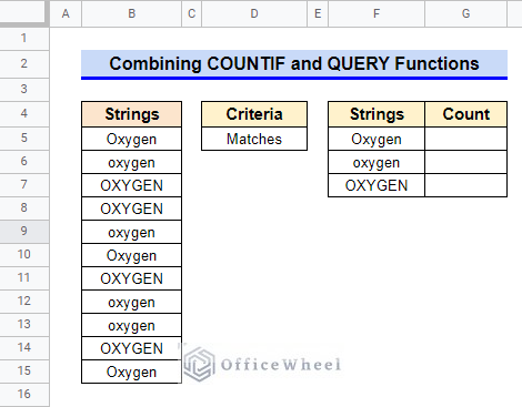
First, let’s get familiar with our dataset. The dataset contains a list of strings that are the same but written in three different cases. Now, let’s count the frequency of each case.
1. Combining COUNTIF, ARRAYFORMULA, ISNUMBER, and FIND Functions
First, let’s combine the COUNTIF, ARRAYFORMULA, ISNUMBER, and FIND functions to execute a case sensitive COUNTIF operation. The FIND function can return the position of a string first found within a text value. Since the search key string and text to be searched are the same here, the FIND will return position 1 whenever a match is found. Later, the COUNTIF function can easily count the number of 1 values in the range.
Steps:
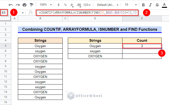
- Firstly, select Cell E5.
- Afterward, type in the following formula-
=COUNTIF(ARRAYFORMULA(ISNUMBER(FIND(D5,$B$5:$B$15))*1),1)- Then, get the required output by pressing Enter key.
Formula Breakdown
- FIND(D5,$B$5:$B$15)
Firstly, the FIND function returns the position of the search key (the content of Cell D5) in each cell of the range B5:B15. Since the search key string and text to be searched are the same here, the FIND will return position 1 whenever a match is found. Else, it will return the #VAULE error.
- ISNUMBER(FIND(D5,$B$5:$B$15)
Here, the ISNUMBER function is for converting the #VALUE to 0 and any number to 1.
- ARRAYFORMULA(ISNUMBER(FIND(D5,$B$5:$B$15))*1)
The ARRAYFORMULA function helps the non-array function ISNUMBER to deal with and display an array.
- COUNTIF(ARRAYFORMULA(ISNUMBER(FIND(D5,$B$5:$B$15))*1),1)
Finally, the COUNTIF function calculates the number of 1 values in the array displayed by the ARRAYFORMULA function.
- At this time, select Cell E5 again and hover your mouse pointer above the bottom-right corner of the selected cell.
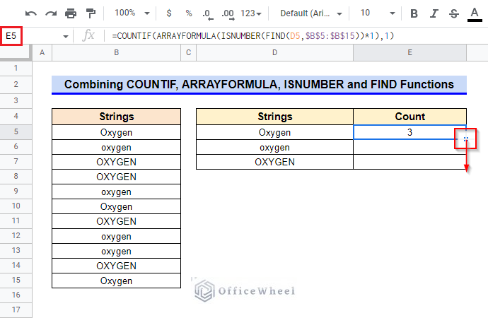
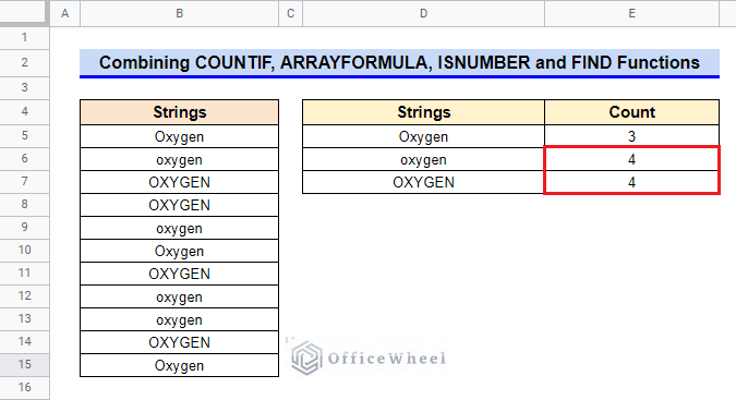
- The Fill Handle icon will be visible at this point. Use it to copy the formula to other cells of Column E.
Read More: [Fixed!] COUNTIF Function Is Not Working in Google Sheets
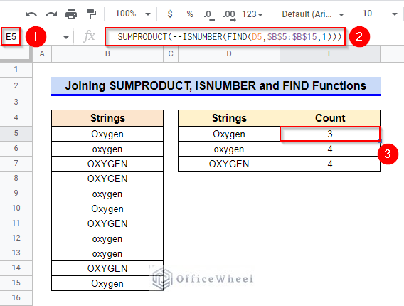
2. Joining SUMPRODUCT, ISNUMBER, and FIND Functions
We can perform the tasks of the COUNTIF and ARRAYFORMULA functions using the SUMPRODUCT function. It can return the sum of the products of analogous entries in two similar-sized ranges.
Steps:
- First, activate Cell E5 by double-clicking on it.
- Then, insert the following formula-
=SUMPRODUCT(--ISNUMBER(FIND(D5,$B$5:$B$15,1)))- Consequently, press Enter key to get the required result.
- Finally, copy the formula to other cells by using the Fill Handle icon.
Formula Breakdown
- FIND(D5,$B$5:$B$15,1)
To start, the FIND function provides the position of the search key (the content of Cell D5) in each cell of the range B5:B15. Since the search key string and text to be searched are the same here, the FIND will return position 1 whenever a match is found. Otherwise, it will return the #VAULE error.
- ISNUMBER(FIND(D5,$B$5:$B$15,1)
Afterward, the ISNUMBER function converts the #VALUE to 0 and any number to 1.
- SUMPRODUCT(–ISNUMBER(FIND(D5,$B$5:$B$15,1)))
Consequently, the SUMPRODUCT function returns the sum of the products of the two equal-sized arrays.
Read More: Google Sheets Count Cells from Another Workbook with COUNTIF Function
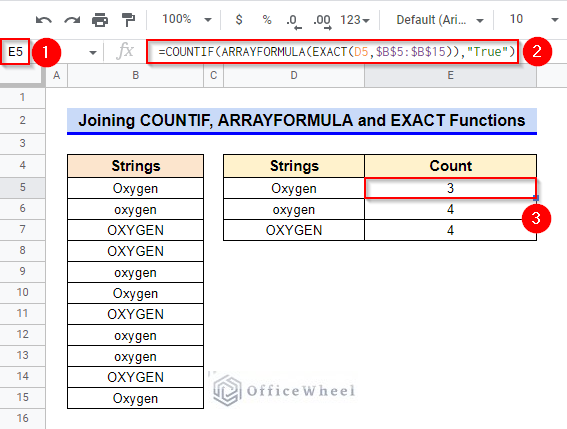
3. Joining COUNTIF, ARRAYFORMULA, and EXACT Functions
One of the limitations of the FIND function is that it corresponds to partial matches. For example, although the “car” and “oscar” words are not an exact match, the FIND function will return a position in this scenario. Therefore, we’ll use the EXACT function as an alternative to the combination of ISNUMBER and FIND functions. It can return the check whether two text values are equal or not. Now, let’s get started.
Steps:
- First, select Cell E5 and then type in the following formula-
=COUNTIF(ARRAYFORMULA(EXACT(D5,$B$5:$B$15)),"True")- Afterward, press Enter key to get the required count.
- Finally, use the Fill Handle icon to copy the formula to other cells of Column E.
Formula Breakdown
- EXACT(D5,$B$5:$B$15)
First, the EXACT function checks whether the strings in Cell D5 and each cell in range B5:B15 are identical or not. If the strings are identical, the EXACT function returns True, or else it returns False.
- ARRAYFORMULA(EXACT(D5,$B$5:$B$15))
Here, the ARRAYFORMULA function helps the non-array function EXACT to deal with and display an array.
- COUNTIF(ARRAYFORMULA(EXACT(D5,$B$5:$B$15)),”True”)
Finally, the COUNTIF function returns the count of True entries in the array displayed by the ARRAYFORMULA function.
Read More: How to Use COUNTIF for Cells Not Equal to Text in Google Sheets
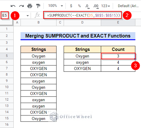
4. Merging SUMPRODUCT and EXACT Functions
Now, let’s execute the EXACT function merged with the SUMPRODUCT function. The SUMPRODUCT function will substitute the COUNTIF and ARRAYFORMULA functions here.
Steps:
- Active Cell E5 by selecting it first and then pressing the F2 function key.
- Afterward, type in the following formula-
=SUMPRODUCT(--EXACT(D5,$B$5:$B$15))- Next, get the required value by pressing the Enter key.
- Consequently, use the Fill Handle icon to copy the formula in other cells.
Formula Breakdown
- EXACT(D5,$B$5:$B$15)
To start, the EXACT function checks whether the strings in Cell D5 and each cell in range B5:B15 are identical or not. If the strings are identical, the EXACT function returns True, or else it returns False.
- SUMPRODUCT(–EXACT(D5,$B$5:$B$15))
Finally, the SUMPRODUCT function returns the sum of the products of the two similar-sized arrays returned by the EXACT functions.
Read More: How to Use COUNTIF for True Condition in Google Sheets
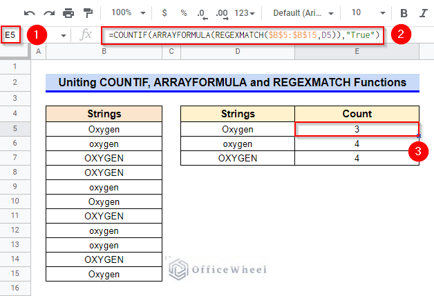
5. Uniting COUNTIF, ARRAYFORMULA, and REGEXMATCH Functions
Another alternative to the FIND function is the REGEXMATCH function. It can also return whether a piece of string matches a regular text value. Here, we’ll combine it with COUNTIF and ARRAYFORMULA functions. You can join the SUMPRODUCT function instead.
Steps:
- Firstly, select Cell E5.
- Insert the following formula next-
=COUNTIF(ARRAYFORMULA(REGEXMATCH($B$5:$B$15,D5)),"True")- Afterward, get the required output by pressing Enter key.
- Finally, use the Fill Handle icon to copy the formula to other cells.
Formula Breakdown
- REGEXMATCH($B$5:$B$15,D5)
First, the REGEXMATCH function checks whether the strings in Cell D5 and each cell in range B5:B15 are identical or not. If the strings are identical, the REGEXMATCH function returns True, or else it returns False.
- ARRAYFORMULA(REGEXMATCH($B$5:$B$15,D5))
Here, the ARRAYFORMULA function helps the non-array function REGEXMATCH to deal with and display an array.
- COUNTIF(ARRAYFORMULA(REGEXMATCH($B$5:$B$15,D5)),”True”)
Finally, the COUNTIF function returns the count of True entries in the array displayed by the ARRAYFORMULA function.
Read More: How to Use COUNTIF Function with OR Logic in Google Sheets
6. Combining COUNTIF and QUERY Functions
We can use the QUERY function to get a range for an exact match in the COUNTIF function. We need to change the dataset to the following for this example.
Steps:
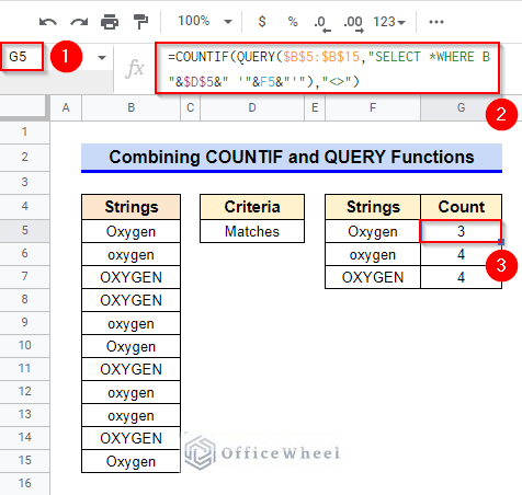
- First, select Cell G5 and type in the following formula-
=COUNTIF(QUERY($B$5:$B$15,"SELECT *WHERE B "&$D$5&" '"&F5&"'"),"<>")- Press Enter key later to get the required count.
- Finally, use the Fill handle icon to copy the formula to other cells of Column G.
Formula Breakdown
- QUERY($B$5:$B$15,”SELECT *WHERE B “&$D$5&” ‘”&F5&”‘”)
First, the QUERY function runs a Google Visualization API Query Language query across the range B5:B15. The expression SELECT * WHERE starts a query. Next expression B indicates the query run in Column B. And the expression “&$D$5&” indicates the query operator. The & symbols are used for extracting the text from Cell D5. The expression ‘“&F5&”’ indicates the cell reference of the search term. The apostrophes (‘’) symbol differentiates the search term from the search operator.
- COUNTIF(QUERY($B$5:$B$15,”SELECT *WHERE B “&$D$5&” ‘”&F5&”‘”),”<>”)
Later, the COUNTIF function counts the number of non-empty cells returned by the QUERY function.
Read More: Use COUNTIF If Cell Contains Specific Text in Google Sheets
Things to Be Considered
- One of the limitations of the FIND function is that it corresponds to partial matches. For example, although the “car” and “oscar” words are not an exact match, the FIND function will return a position in this scenario.
Conclusion
This concludes our article to learn how to execute case sensitive COUNTIF in Google Sheets. I hope the demonstrated examples were ideal for your requirements. Feel free to leave your thoughts on the article in the comment box. Visit our website OfficeWheel.com for more helpful articles.
Related Articles
- Google Sheets Add Calculated Field for Pivot Table with COUNTIF
- COUNTIF Function with “Not Equal to” Criterion in Google Sheets
- Use COUNTIF Function to Count Checkbox in Google Sheets
- COUNTIF with Greater than and Less than Criteria in Google Sheets
- How to Use VLOOKUP with COUNTIF Function in Google Sheets