We often need to get the result of a particular task in the fastest possible way. Like, if an employee of a company has a dataset containing records of all the workers like their attendance, average working hours, and much more, and if he wants to see all the records of a particular worker, he doesn’t have time to walk through the whole dataset and find them one by one. So what can he do? He can combine some amazing formulas like IF, INDEX, MATCH, VLOOKUP, COUNTIF and much more to get his desired result within the shortest possible time. In this article, we have demonstrated some examples on how to use VLOOKUP with COUNTIF function in Google Sheets.
A Sample of Practice Spreadsheet
You can download the spreadsheet used to demonstrate examples in this article.
4 Ideal Examples to Use VLOOKUP with COUNTIF Function in Google Sheets
We can use the VLOOKUP and COUNTIF functions in many ways. Here we have described 4 usual examples that are necessary from many perspectives.
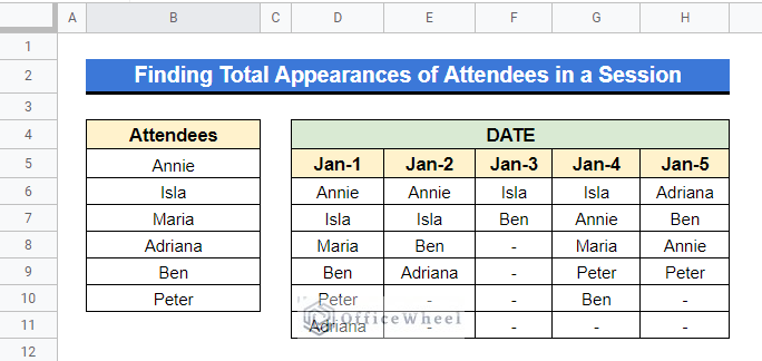
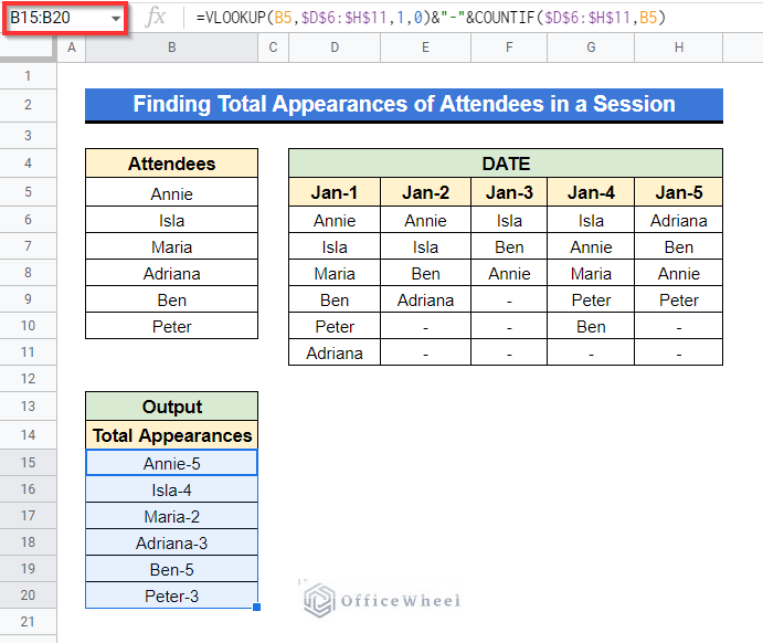
Example 1. Finding Total Appearances of Attendees in a Session
Let’s assume, the following dataset is containing the records of 6 attendees’ appearances of a 5-day session on a particular topic. We want to calculate the total appearances of each attendee in that session using VLOOKUP and COUNTIF functions.
Steps:
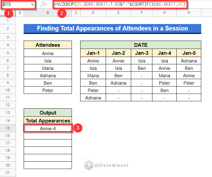
- First, select Cell B15 and then apply the following formula below and press Enter–
=VLOOKUP(B5,$D$6:$H$11,1,0)&"-"&COUNTIF($D$6:$H$11,B5)- Here, we can see in Cell B15 that the total number of appearances of attendee “Annie” is 4.
Formula Breakdown
- COUNTIF($D$6:$H$11,B5)
Counts the total number of presence that is given input in Cell B5 within Cell range D6:H11.
- VLOOKUP(B5,$D$6:$H$11,1,0)
Looks for value in Cell B5 within Cell range D6:H11 and returns the corresponding value from Column D if the lookup value exists within that range.
- VLOOKUP(B5,$D$6:$H$11,1,0)&”-“&COUNTIF($D$6:$H$11,B5)
Finally, the & operator will join the outputs with a hyphen.
- Now if I input “Annie” in a different cell within Cell range D6:H11, the total number of appearances will be changed. Like, if I input “Annie” in Cell F8 then see what happens!
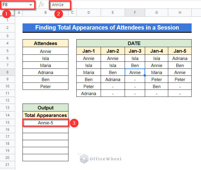
- The total number of appearances of “Annie” is now 5.
- Now, simply drag down using the Fill Handle icon as shown in the circled portion.
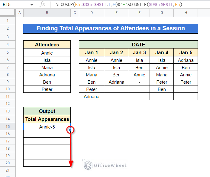
- And you will get the total number of appearances of the other attendees as well.
Read More: Google Sheets Count Cells from Another Workbook with COUNTIF Function
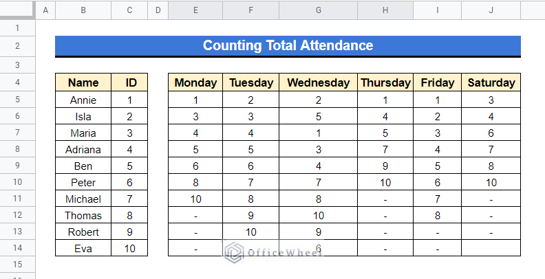
Example 2. Counting Total Attendance
Suppose, in the following dataset, one-week attendance record of some students is given along with their ID number. What we want to know is the total attendance of a particular student within just a moment.
Steps:
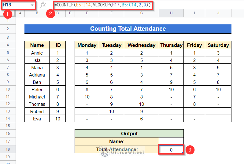
- In the following dataset, select Cell H18 and apply the formula given below then press Enter–
=COUNTIF(E5:J14,VLOOKUP(H17,B5:C14,2,0))- Here we can see what appears in Cell H18 is “0”. It’s because nothing is given in Cell H17 as input.
Formula Breakdown
- VLOOKUP(H17,B5:C14,2,0)
After giving input in Cell H17 the VLOOKUP function will look for that value within Cell range B5:C14. Then it will match the corresponding number for the input in Cell H17. Like if we input “Robert” then the function will match with its corresponding number that is “9”.
- COUNTIF(E5:J14,VLOOKUP(H17,B5:C14,2,0))
The number produced by the VLOOKUP function within the Cell range E5:J14 is counted using the COUNTIF function.
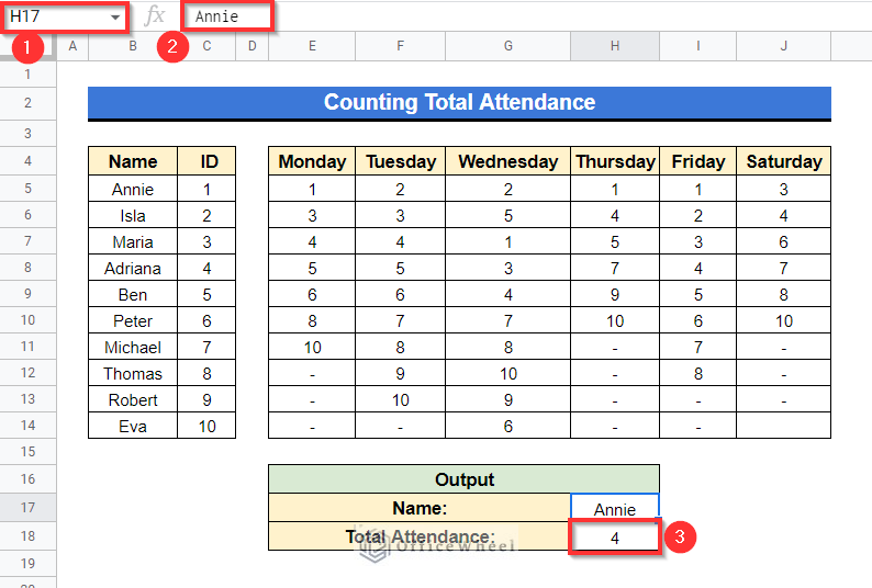
- Now, if you type down one of the students’ names in Cell H17, the total number of attendances of that student will appear in Cell H18. Like, if you type down “Annie” in Cell H17 the total number of attendances of “Annie” will appear in Cell H18 and that will be “4”.
Read More: [Fixed!] COUNTIF Function Is Not Working in Google Sheets
Similar Readings
- How to Execute Case Sensitive COUNTIF in Google Sheets
- Google Sheets Add Calculated Field for Pivot Table with COUNTIF
- How to Use COUNTIF Function with OR Logic in Google Sheets
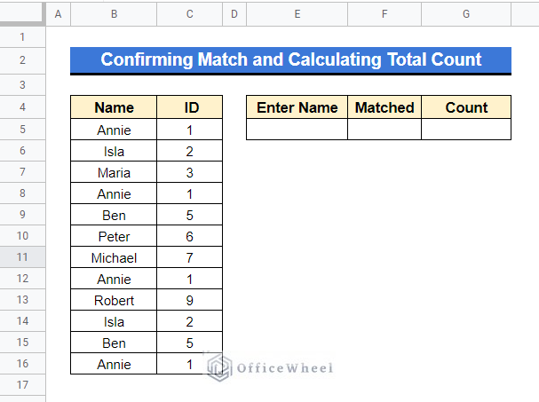
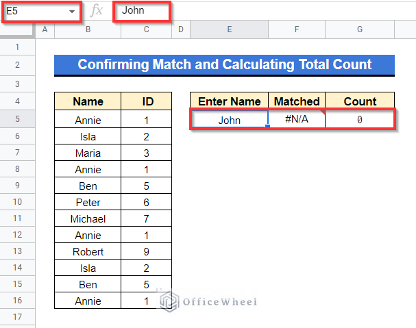
Example 3. Confirming Match and Calculating Total Count
Presume, we have a dataset of some students with their ID. What we want to check is whether a student is on the dataset list or not and if he exists then what count of that particular student is present in the dataset?
Steps:
- In the following dataset, select Cell F5 then apply the following formula-
=VLOOKUP(E5,$B$5:B,1,0)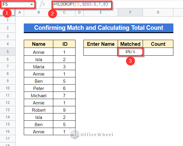
- As nothing is typed down yet in Cell E5, that’s why the match is shown as “#N/A”.
- Now apply the following formula in Cell G5 and then press Enter–
=COUNTIF($B$5:B,E5)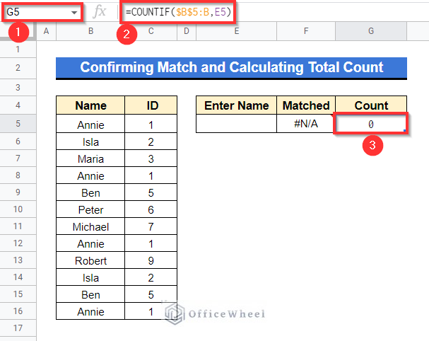
- The result is showing “0” as no input is given in Cell E5.
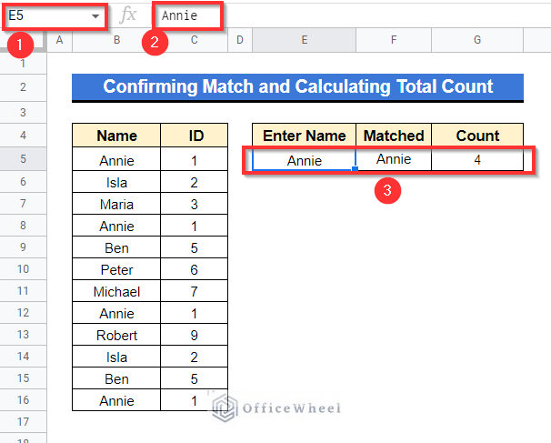
- Now type down any name from the list or outside the list in Cell E5 and it will show satisfactory results. Like if you type down “Annie” in Cell E5 then it will show “Annie” in Cell F5 and the total number of counts for “Annie” will be shown “4” in Cell F5 as the name “Annie” is on the list about 4 times.
- And if we input a random name that is not on the list, then the result will be as follows-
Read More: COUNTIF Function with “Not Equal to” Criterion in Google Sheets
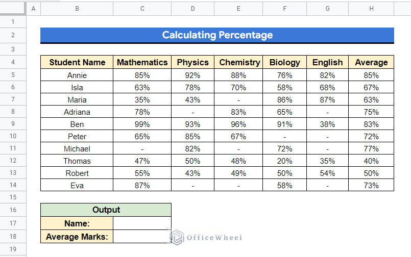
Example 4. Calculating Percentage
Let’s assume, we have a dataset of grade sheets of some students. Now, if there are at least 3 percentages for each grade, our target is to get their average percentage. That means if any student has more or equal to 3 percentages, the result will be the average percentage. If any student has less than 3 percentages, then the result will return as “#N/A”. We will be using the combination of VLOOKUP, COUNTIF, IF, INDEX, MATCH and NA functions.
Steps:
- First, select Cell C18, apply the following formula and press Enter–
=IF(COUNTIF(INDEX($C$5:$G$14,MATCH(C17,$B$5:$B$14,0),0),">0")<3,NA(),VLOOKUP(C17,$B$5:$H$14,7,0))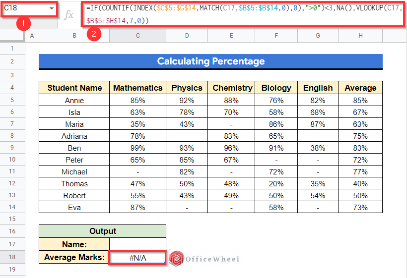
Formula Breakdown
- VLOOKUP(C17,$B$5:$H$14,7,0)
Looks for the value in Cell C17 within Cell range B5:H14 and return the corresponding value for Cell C17 from column 7. And if false then it will return “0”.
- NA()
Returns an error as “#N/A” if the value is not available.
- MATCH(C17,$B$5:$B$14,0)
Will return the corresponding value of Cell C17 that is within Cell range B5:B14.
- INDEX($C$5:$G$14,MATCH(C17,$B$5:$B$14,0),0)
This formula works as INDEX($C$:$B$5,5,0) which is basically the set of percentages corresponding to Cell C17.
- COUNTIF(INDEX($C$5:$G$14,MATCH(C17,$B$5:$B$14,0),0),”>0″)
This counts the occurrences of percentages for the lookup value.
- IF(COUNTIF(INDEX($C$5:$G$14,MATCH(C17,$B$5:$B$14,0),0),”>0″)<3,NA(),VLOOKUP(C17,$B$5:$H$14,7,0))
Returns back the typical proportion for Cell C17 in Column 8 for the condition “<3”.
- What we can see is the result returned as “#N/A”. This is because no such entry is given in Cell C17.
- Now, suppose we want to know the average percentage result of a student named “Maria”. Simply type down “Maria” in Cell C17 and press Enter-
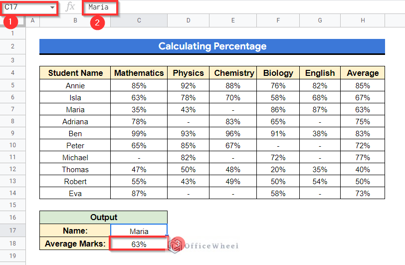
- We can see that the average percentage mark of “Maria” is “63%”. The result returned as an average percentage form as “Maria” has 4 percentages of 4 subjects which is obviously greater than 3.
- Now, we will type down “Eva” in Cell C17, and let’s see what happens-
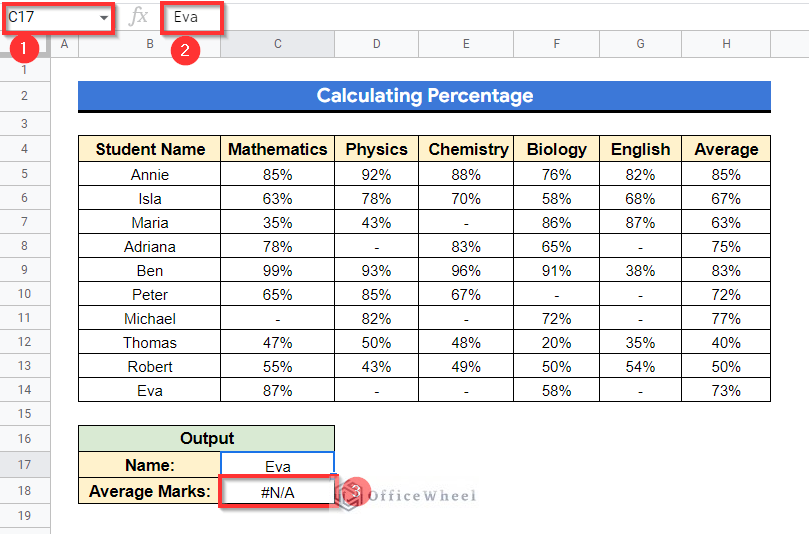
- The result returned as “#N/A” because “Eva” has only percentages of 2 subjects which is less than 3.
Read More: COUNTIF with Greater than and Less than Criteria in Google Sheets
Conclusion
We can solve almost all the time-consuming tasks within the shortest possible time in Google Sheets or Excel. Using VLOOKUP and COUNTIF is just a small part of that. In this article, we have described 4 ideal examples on how you can use VLOOKUP with COUNTIF in Google Sheets. Hope this will help you with your task. Visit our site officewheel.com to see more related articles.