In Google Sheets, the Pivot Table can be a very useful tool to summarize a huge dataset. To analyze data, you can insert any general function from the Pivot table editor. Moreover, you can also customize any formula in the Calculated Field option. In this article, we will explain the pivot table calculated field for COUNTIF in Google Sheets.
A Sample of Practice Spreadsheet
You can download Google Sheets from here and practice very quickly.
Steps to Add Calculated Field with COUNTIF Formula for Pivot Table in Google Sheets
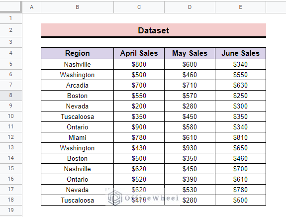
As the COUNTIF function is not placed in the pivot table formulas, so we have to customize the COUNTIF formula. To do so, before going to the main steps we have to create a dataset that represents sales of the different regions for different months. Here we develop columns namely: Region, April Sales, May Sales, and June Sales.
Step 1: Creating Pivot Table
After developing the dataset to create a pivot table,
- First, go to the Insert bar and select the Pivot table option.
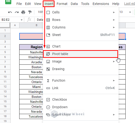
- After clicking on the Pivot table option, you will find the Create pivot table box.
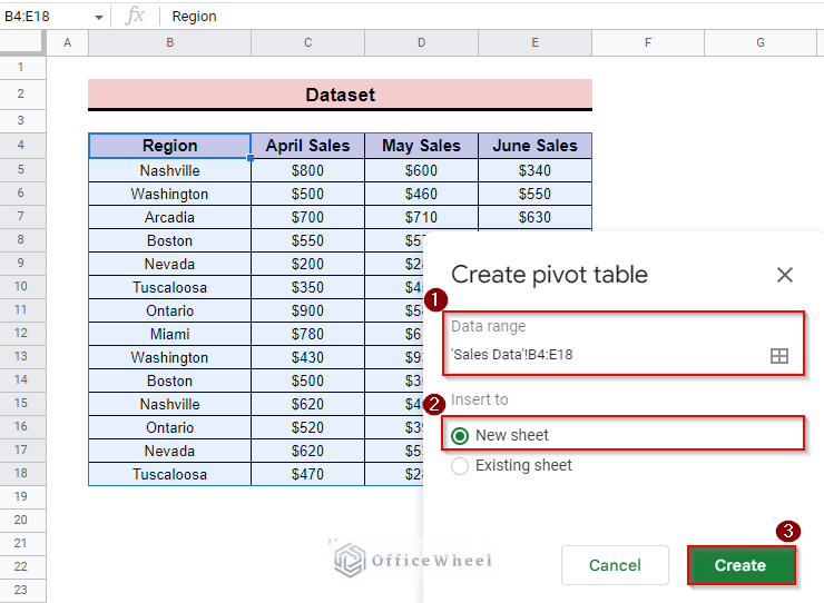
- Now input the Data range and Insert to. Here we add the entire dataset as the Data range and for Insert to option select the New sheet option.
- Then press on Create.
- Immediately, you will find a new sheet name Pivot table is created.
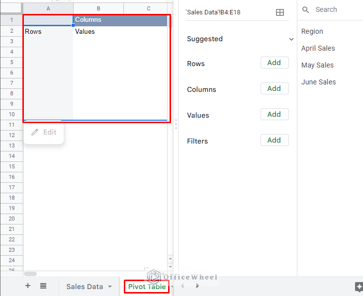
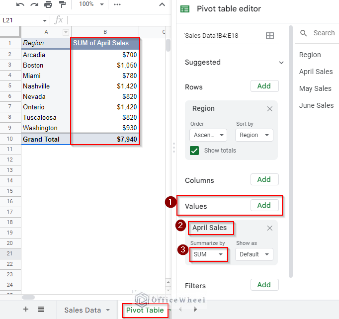
- Now you can add any rows, columns, or values in the table. Here, we first add the Region as Rows.
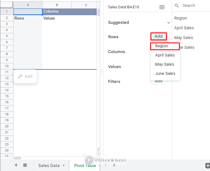
- After adding the Region from the list, you will find it in the main table.
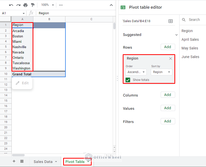
Step 2: Setting Up Values in Pivot Table
This is just an example of how we can add column values in a pivot table. This step is optional.
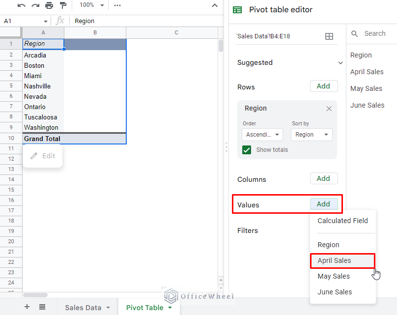
You can insert any formulas in the table by using the Values bar. For this,
- First, go to the Values option select Add and click on any title that you want to insert. Here, we select the April Sales option.
- Then for the Summarized by option select the SUM formula. And you will find the Sum of April Sales automatically add to the Region column.
- You can also apply all these formulas in the table and get your desired result.
Similar Readings
- How to Execute Case Sensitive COUNTIF in Google Sheets
- Use COUNTIF Function with OR Logic in Google Sheets
- COUNTIF with Greater than and Less than Criteria in Google Sheets
- Google Sheets Count Cells from Another Workbook with COUNTIF Function
Step 3: Inserting Calculated Field with COUNTIF Formula
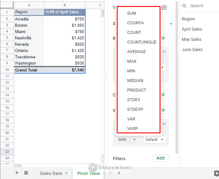
Now for the meat of our article. As we can see in the last image, in the formula list the COUNTIF formula is not available. But you can also resolve this problem and easily apply the COUNTIF formula in Google Sheets by using the Calculated Field. To do so,
- First, go to the Values and click on Add. then select the Calculated Field option.
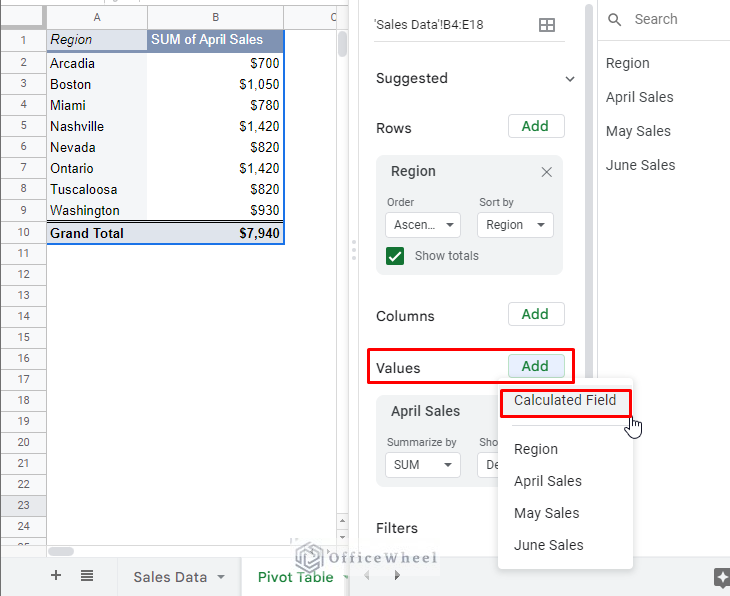
- After clicking on the Calculated Field, a column automatically adds to the table, and you can find a Formula bar where you can apply the customized formula.
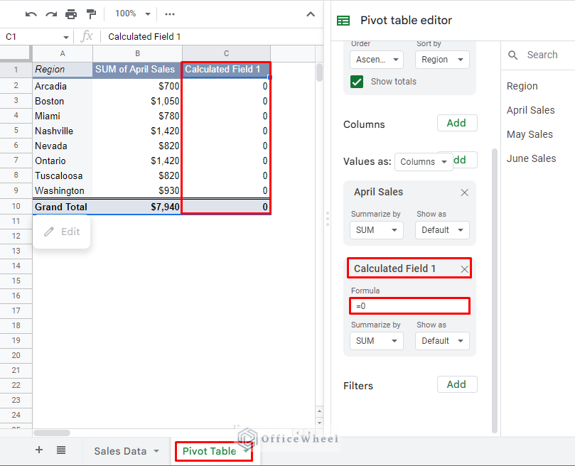
- Now insert the COUNTIF formula in the Formula bar.
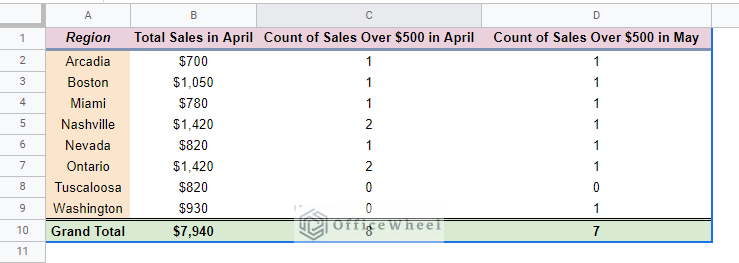
=COUNTIF(‘April Sales’,”>$500”)- Here, we are trying to count the number of Sales greater than $500 for April.
- We do not get the correct results yet, so we must make one more change.
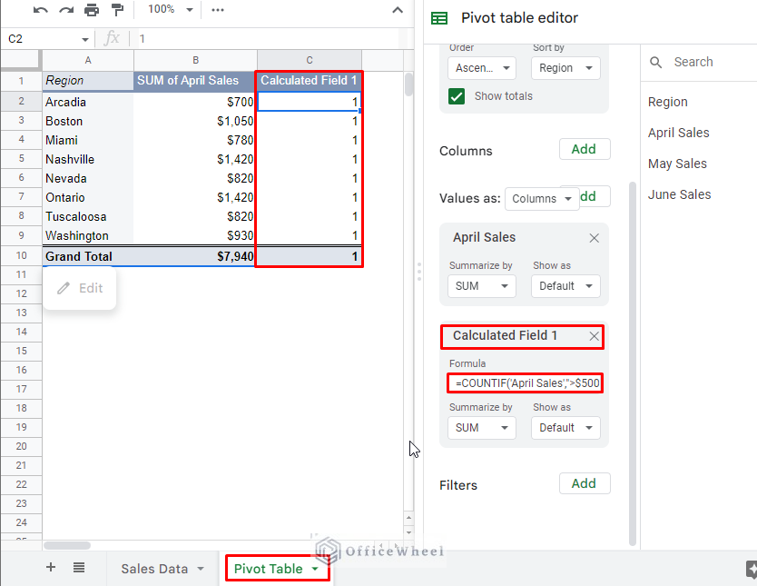
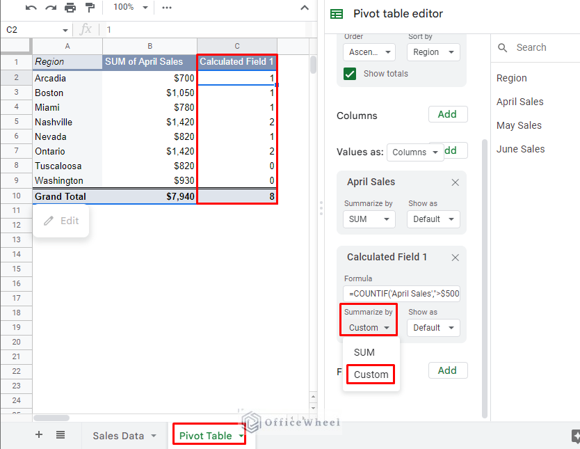
- Then select the Custom option from the Summarized by drop-down.
Read More: [Fixed!] COUNTIF Function Is Not Working in Google Sheets
Step 4: Finalizing Outcome
- Finally, you can find the output of the COUNTIF formula in the Calculated Field 1 column.
- With Custom selected, the pivot table will automatically update the results in the column.
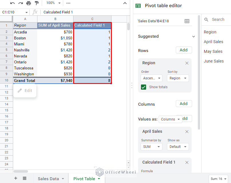
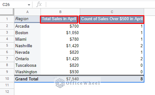
- You can further customize the column by changing the heading.
- This can be done by double-clicking on the column heading to edit the text.
- Here we change the two-value column title and insert “Total Sales in April” and “Count of Sales over $500 in April”.
- Additionally, by applying the same process we add the count of sales over $500 for the month of May.
=COUNTIF('May Sales',">$500")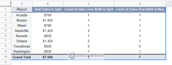
Read More: How to Use VLOOKUP with COUNTIF Function in Google Sheets
Things to Remember
- Careful about inserting values and formulas.
- In the custom formula use a single quotation for the column heading.
Conclusion
We believe this article will help you to get a clear concept of the Google Sheets pivot table calculated field by using the COUNTIF formula. To explore more about pivot tables in google sheets you can visit the OfficeWheel website.