Google Sheets Copy Conditional Formatting but Change Reference Cell

Conditional formatting is a very dynamic feature in Google Sheets. It enables us to format our dataset with the criteria we put. Sometimes we need to apply the same conditional formatting again and again to different ranges. But if we don’t change the reference cell when applying the conditional formatting repeatedly, then it will give an erroneous result. So in this article, we’ll see 3 suitable methods to copy conditional formatting but change the reference cell in Google Sheets with clear steps and images.

A Sample of Practice Spreadsheet

You can download Google Sheets from here and practice very quickly.

3 Suitable Methods to Copy Conditional Formatting but Change Reference Cell in Google Sheets

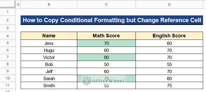
Let’s get introduced to our dataset first. Here we have some students’ names in Column B, their Math scores in Column C, and their English scores in Column D. We have applied a condition in Column C. The condition is that if the Math score in any cell of Column C is above 60 then that cell will be highlighted with the green color. Now we want to copy this conditional formatting into Column D which has the English Score. So we have to change the cell reference. I’ll show you 3 suitable methods to copy conditional formatting but change the reference cell in Google Sheets with the help of this dataset.

1. Applying Paste Special Command

First of all, we can apply the Paste Special command to copy conditional formatting into another range. This method changes the cell reference automatically. This command has 2 distinct sub-commands. One is the Format Only command and the other is the Conditional Formatting Only command. We’ll discuss them below.

1.1. Using Format Only Command

Earlier on we’ll see the steps regarding the Format Only command.

Steps:

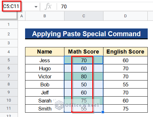
• Firstly, select all cells from Cell C5 to C11 and press Ctrl+C from the keyboard to copy the cells.

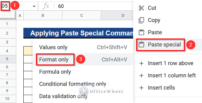
• Secondly, select Cell D5 and put Right-Click on the mouse.
• Then, go to Paste Special > Format Only.

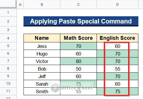
• Finally, you’ll see that we have copied the conditional formatting in Column D and the reference cell is changed automatically.

1.2. Assigning Conditional Formatting Only Command

Now, we’ll see the application of the Conditional Formatting Only command.

Steps:

• At first, copy all the cells from Cell C5 to C11 by selecting them and pressing Ctrl+C from the keyboard.

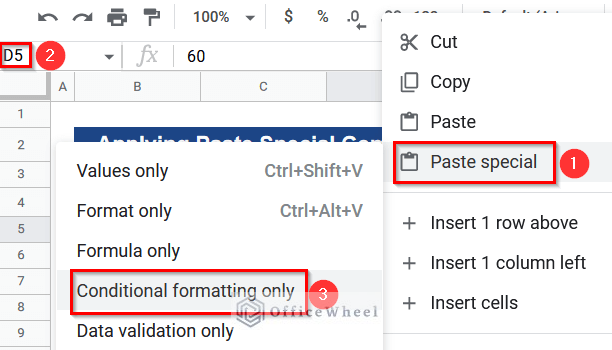
• Next, select Cell D5 and give Right-Click on the mouse.
• After that, go to Paste Special > Conditional Formatting Only.

• Ultimately, you’ll find that the conditional formatting is copied in Column D.

2. Using Paint Format Command

The Paint Format command directly copies the conditional formatting from one range to another range. This method has fewer steps than the previous method. Let’s see the steps.

Steps:

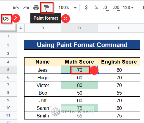
• First of all, select Cell C5 and click on the Paint Format button.

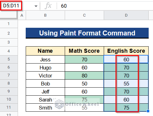
• At last, select the cells from Cell D5 to D11 and the conditional formatting will be copied with the changed reference cells in Column D very quickly.

3. Copying Conditional Formatting Formula

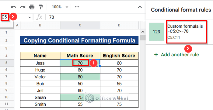
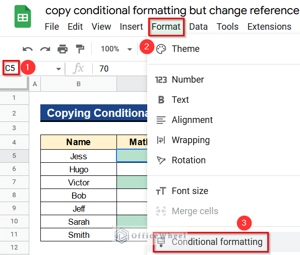
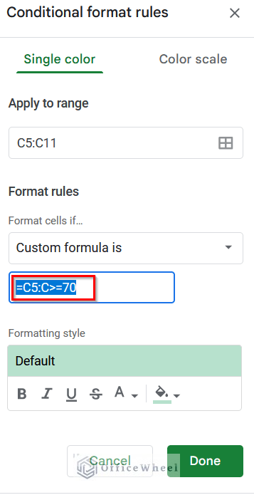
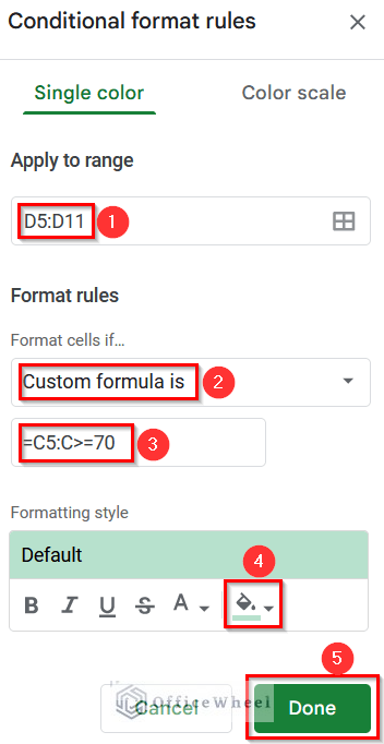
At present we have applied a custom formula with conditional formatting to Column C of our dataset as you can see in the picture. The formula is-

It means that the cells of Column C will be highlighted with the green color if any cell has a value greater or equal to 70. Again we want to copy this conditional formatting with the formula in Column D. Let’s see how to copy conditional formatting with keeping the formula but changing the reference cell in Google Sheets.

Steps:

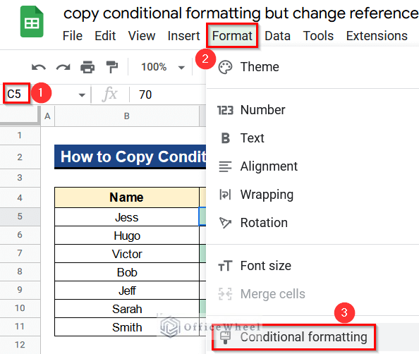
• In the beginning, select Cell C5 and go to Format > Conditional Formatting.

• In the Conditional Format Rules window copy the following formula from the formula box by pressing Ctrl+C together-

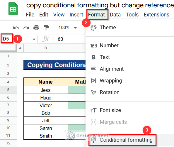
• Again, select Cell D5 and go to Format > Conditional Formatting.

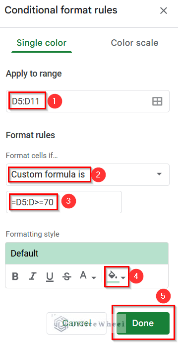
• Afterward, change the cell range from Cell D5 to D11 under Apply to Range menu.
• Consequently, select Custom Formula Is under the Format Rules menu and paste the copied rule in the formula box by pressing Ctrl+V. Finally, replace C with D. So the formula will then look like as follows:

• Moreover, select the green color from the Color button and click on the Done button.

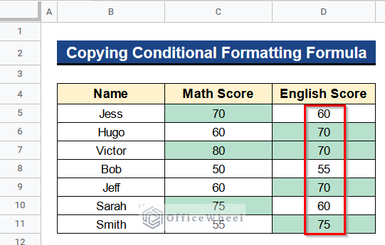
• In the end, you’ll get your desired output. The scores above or equal to 70 will be highlighted in Column D.

How to Copy Conditional Formatting Based on Another Cell in Google Sheets

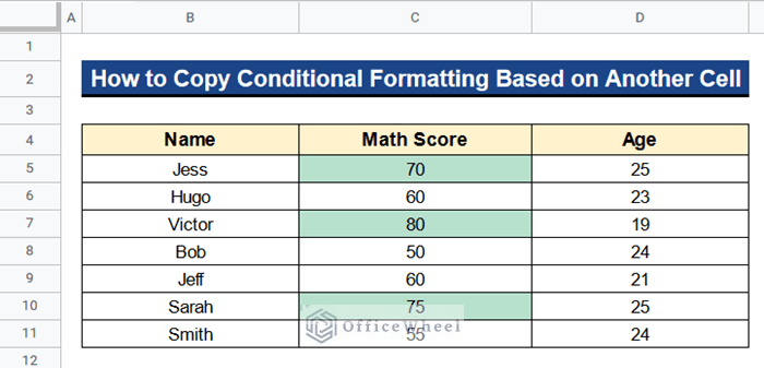
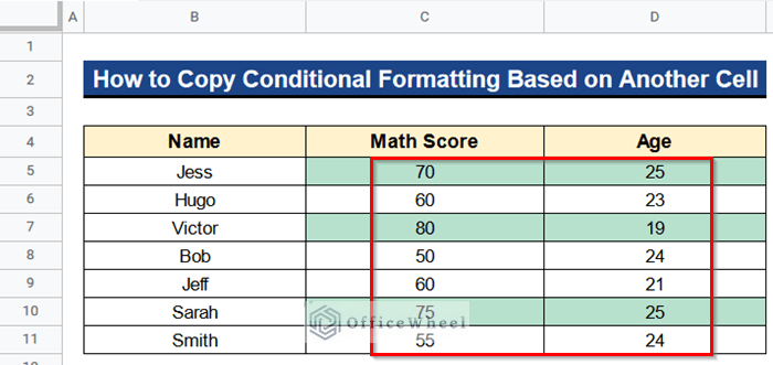
We have a slightly different problem now. There are some students’ names in Column B, their Math scores in Column C, and their ages in Column D. I highlighted Column C in a way that any value greater or equal to 70 will be highlighted in green color. For this purpose, we have applied a formula with conditional formatting in Column C. Now we want to copy this conditional formatting in Column D based on the cells of Column C. So, let’s see the steps to copy conditional formatting based on another cell in Google Sheets.

Steps:

• Before all, select Cell C5 and go to Format > Conditional Formatting.

• Further, copy the following formula from the Conditional Format Rules window by pressing Ctrl+C together-

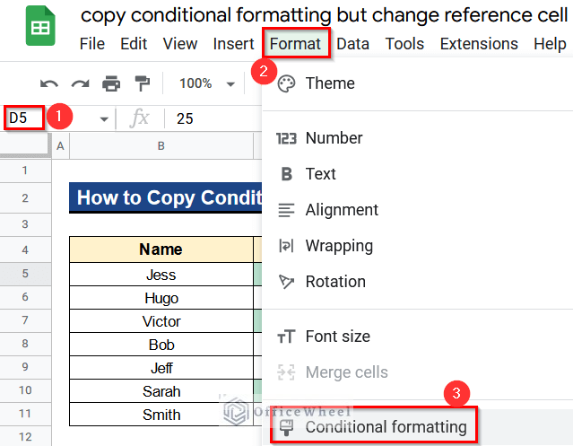
• Apart from this, select Cell D5 and go to Format > Conditional Formatting.

• Also, put the cell range from Cell D5 to D11 under the Apply to Range menu.
• Besides, select Custom Formula Is under the Format Rules menu and paste the following formula into the formula box by pressing Ctrl+V together-

• Subsequently, select the green color from the Color button.
• Then, click on the Done button.

• Finally, you’ll see that we have copied the conditional formatting in Column D based on the cells of Column C. That’s why you can see the green color in the corresponding cells of Columns C and D like the picture.

Read More: How to Copy Conditional Formatting to Other Cells in Google Sheets

How to Copy Conditional Formatting from One Sheet to Another Google Sheets

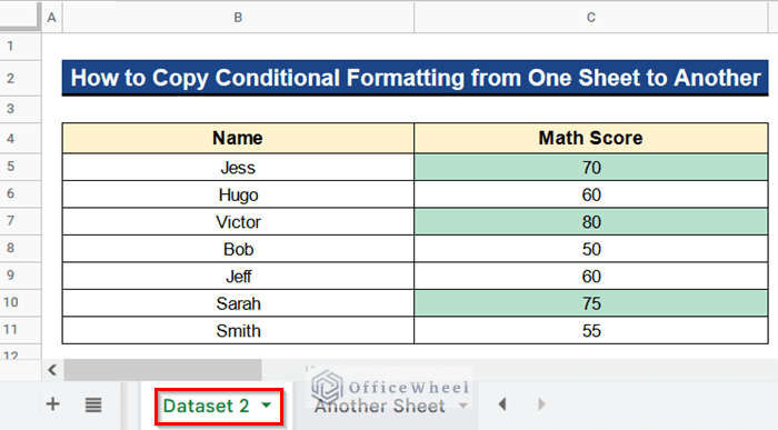
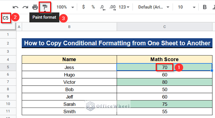
We can further copy the conditional formatting from one sheet to another Google Sheets very easily. Like below in the “Dataset 2” sheet we have some names in Column B and their Math scores in Column C. In addition to that, we have conditional formatting in Column C. This formatting highlights the cells in Column C that have values greater than 60.

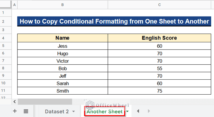
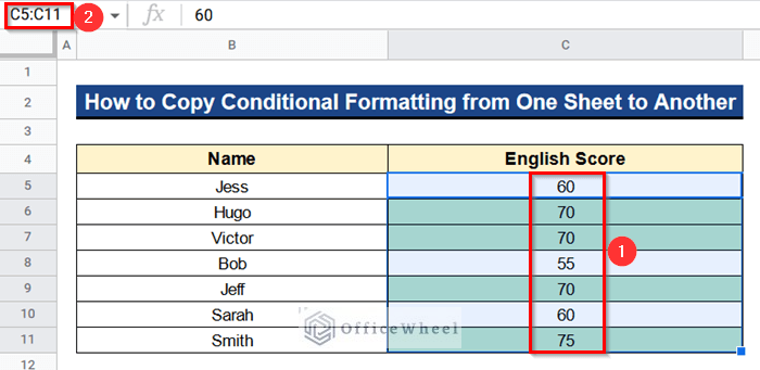
In “Another Sheet” we have English scores instead of Math scores in Column C. Now we want to copy the conditional formatting from the “Dataset 2” sheet to “Another Sheet”.

Steps:

• Initially, select Cell C5 and click on the Paint Format button from “Dataset 2”.

• Ultimately, go to “Another Sheet” and select the cells from Cell C5 to C11.
• You’ll see the highlighted cells of Column C in “Another Sheet”.

Conclusion

That’s all for now. Thank you for reading this article. In this article, I have discussed 3 suitable methods to copy conditional formatting but change the reference cell in Google Sheets. Besides, I have discussed how to copy conditional formatting based on another cell in Google Sheets and from one sheet to another sheet. Please comment in the comment section if you have any queries about this article. You will also find different articles related to google sheets on our officewheel.com. Visit the site and explore more.

Related Article

• Copy Conditional Formatting with Relative Cell References in Google Sheets