Conditional formatting is an awesome tool for highlighting important data in Google Sheets. We can set predefined conditions and highlight the relevant data easily using this tool. Conditional formatting helps to read the data easily with different color formats. In large datasets, we can easily copy the conditional formatting with relative cell references from one range to another in Google Sheets. This saves a lot of time and effort. Follow the article to learn how to do that.
A Sample of Practice Spreadsheet
You can download the practice spreadsheet from the download button below.
2 Simple Ways to Copy Conditional Formatting with Relative Cell References in Google Sheets
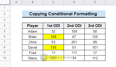
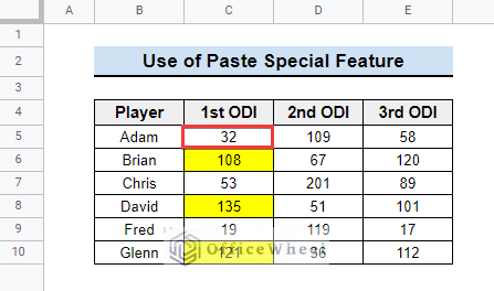
The following dataset shows the scores of six cricket players in 3 ODI matches. Here conditional formatting is applied to the 1st ODI column for centuries. For this dataset, the condition is ‘value is greater than or equal to 100’, and the relative cell reference is C5:C10. We will copy the formatting from this range to the 2nd ODI and 3rd ODI columns.
Follow the methods below to be able to do that.
1. Using Paint Format Tool
The Paint format tool is used to copy the cell formatting from one range to another range. You can easily copy the conditional formatting with relative cell reference using the Paint format tool in google sheets. Follow the simple steps given below.
📌 Steps:
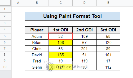
- First, you need to select a cell (C5) from the column where conditional formatting is already applied. You can select any cell or the entire range C5:C10.
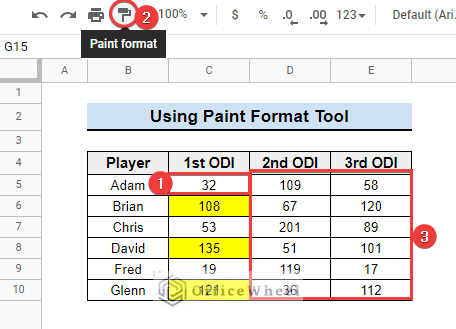
- Then click on the Paint format icon from the quick access toolbar. Next, drag the mouse from cell D5 to E10.
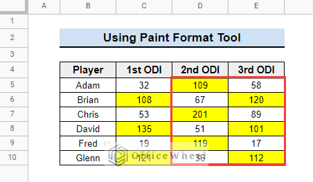
- Finally, you will see that the conditional formatting is copied to the range D5:E10.
2. Utilizing Paste Special Feature
Another easy way to copy conditional formatting is to use the Paste special feature in Google Sheets. Check the simple steps below to be able to do that.
📌 Steps:
- First, copy a cell or the range where conditional formatting is applied. Here we have copied cell C5 just like the previous method. You can press CTRL + C to copy the cell.
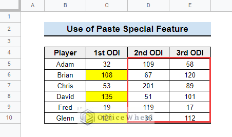
- Then select the range where you want to apply the conditional formatting. You can select the D5:E10 range in this dataset.
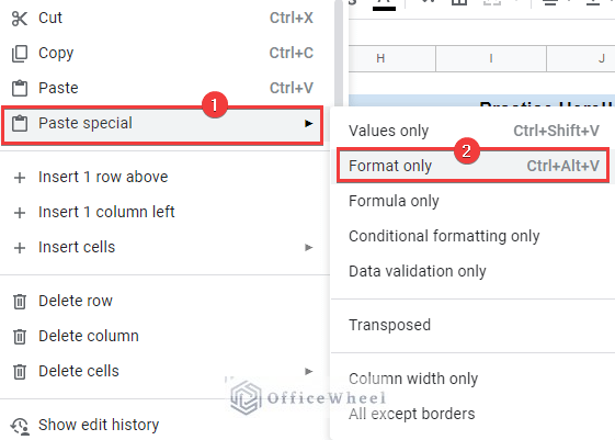
- Next, right-click on the selected range and go to Paste special >> Format only as shown below. Alternatively, you can use the CTRL + ALT + V shortcut to do that.
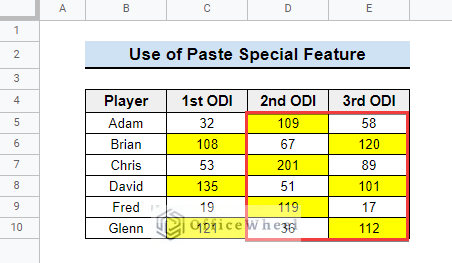
- As a result, the conditional formatting from the 1st ODI column will be copied to the 2nd ODI and 3rd ODI columns as earlier.
Things to Remember
- You need to make sure that the formulas used in the conditional formatting contain relative cell references only. Otherwise, these methods will return erroneous results.
- You can apply the methods to copy the conditional formatting to ranges in other sheets also.
Conclusion
In conclusion, I hope that now you can easily copy conditional formatting with relative cell references in Google Sheets without any hassle. Hopefully, it will help you to visualize your data more properly. Please use the comment section below for further queries or suggestions. You may also visit our OfficeWheel blog to explore more about Google Sheets.