The IFS function returns logical values quickly for multiple criteria in Google Sheets. Whereas this function has a certain limitation. It can only give values when all the conditions are TRUE. On the other hand, this function will return a No Match Error (#N/A) when all conditions are FALSE. In this article, we’ll see 5 useful fixes when the IFS function is returning a No Match Error (#N/A) in Google Sheets with clear images and steps.
A Sample of Practice Spreadsheet
You can download Google Sheets from here and practice very quickly.
5 Useful Fixes When IFS Function Is Returning No Match Error in Google Sheets
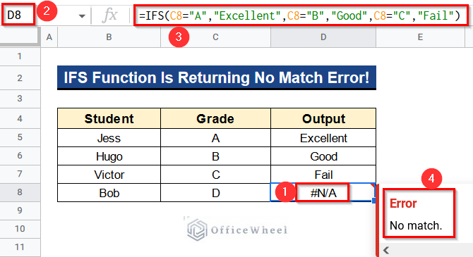
Let’s get introduced to our dataset first. Here we have some students in Column B and their grades in Column C. We wanted to put some comments regarding their grade in Column D. The comments are “Excellent” for grade A, “Good” for grade B, and “Fail” for grade C. So I have applied the following formula in Column D–
=IFS(C5="A","Excellent",C5="B","Good",C5="C","Fail")But it is giving a No Match Error (#N/A) because grade D is not present in our criteria. So I’ll show 5 useful fixes when the IFS function is returning a No Match Error (#N/A) in Google Sheets.
Solution 1. Removing Unwanted Spaces
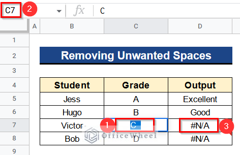
Before all, we’ll look into a silly matter. We might have left some unwanted spaces in our dataset. As you can see in the picture, we have left some spaces in Cell C7. Clearly in this case the formula won’t work. We have to remove those spaces.
Steps:
- Firstly, remove the space manually. Just click on Cell C7 and delete the spaces.
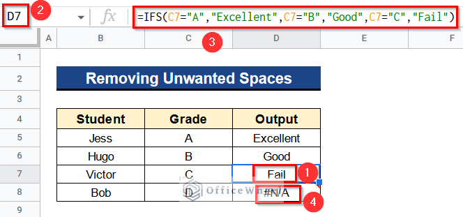
- Then the formula will work just fine.
- It is still showing an error in Cell D8 because grade D is absent from our criteria. We’ll see solutions regarding this in our next methods.
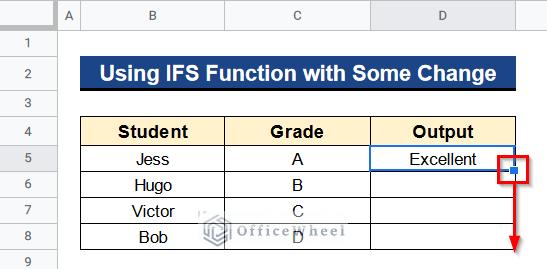
Solution 2. Using IFS Function with Some Change
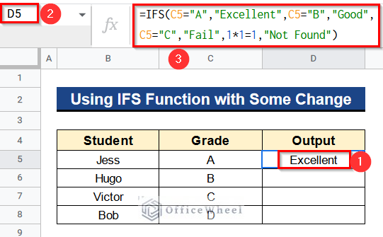
Our formula with the IFS function is returning a No Match Error (#N/A) in Google Sheets in our previous method. Because when the criteria don’t match, this function gives a No Match Error (#N/A). That’s why we’ll make some changes in our formula and you’ll see that then the formula is working fine. We are putting a new condition 1*1=1 and a new value “Not Found” in our formula. This condition means that when the IFS function is not finding any related criteria then it’ll show “Not Found” instead of a No Match Error (#N/A).
Steps:
- At first, type the following formula in Cell D5–
=IFS(C5="A","Excellent",C5="B","Good",C5="C","Fail",1*1=1,"Not Found")- Next, hit Enter to get the output.
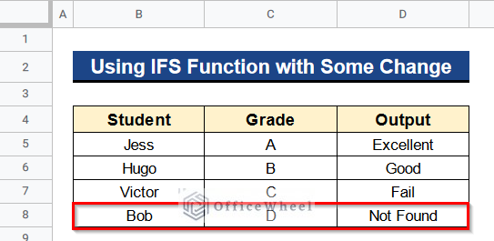
- Finally, you’ll see the comments in all the cells of Column D. As grade D is not present in our condition so it is showing “Not Found” in Row 8.
Read More: How to Use IFS Function in Google Sheets (3 Ideal Examples)
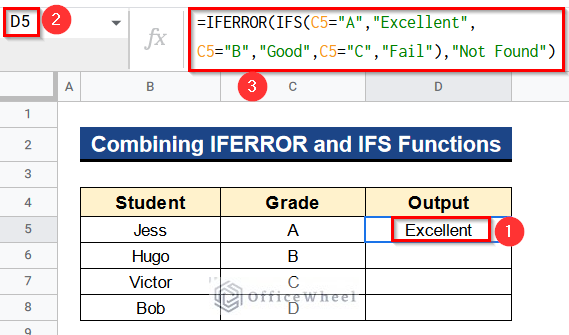
Solution 3. Combining IFERROR and IFS Functions
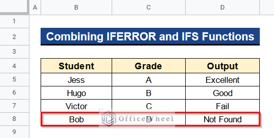
Furthermore, we can combine the IFERROR and IFS functions to get some values when using only the IFS function giving a No Match Error (#N/A). The IFERROR function will give the output as “Not Found” when the conditions are not matching. Thus our problem will be solved.
Steps:
- First of all, write the following formula in Cell D5–
=IFERROR(IFS(C5="A","Excellent", C5="B","Good",C5="C","Fail"),"Not Found")- After that, press Enter to get the result.
Formula Breakdown
- IFS(C5=”A”,”Excellent”, C5=”B”,”Good”,C5=”C”,”Fail”)
Initially, this function searches for values A, B or C in Cell C5 and returns the corresponding comments if the conditions are TRUE. Otherwise, it returns a No Match Error (#N/A).
- IFERROR(IFS(C5=”A”,”Excellent”, C5=”B”,”Good”,C5=”C”,”Fail”),”Not Found”)
Then, this function returns the corresponding comments if the conditions are TRUE. Or it returns the comment “Not Found” as a value.
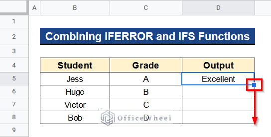
- Consequently, use the Fill Handle tool to apply the formula to all of the cells of Column D.
- At last, the comments are there in all the cells of Column D. You can see “Not Found” in Row 8.
Read More: How to Use IFS Between Two Numbers in Google Sheets
Solution 4. Applying Nested IF Functions
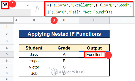
We can use multiple IF functions together to solve multiple criteria in Google sheets. When we use multiple IF functions together it is called nested IF functions. This function returns a value when all criteria are TRUE, and another value when all criteria are FALSE. So nesting multiple IF functions together will resolve our issue.
Steps:
- In the beginning, insert the following formula in Cell D5–
=IF(C5="A","Excellent",IF(C5="B","Good", IF(C5="C","Fail","Not Found")))- After that, click Enter to get the desired output.
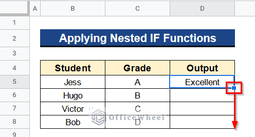
- Again, assign the Fill Handle tool to the rest of the cells of Column D.
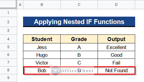
- At last, you’ll find your desired output in Column D. In Row 8 you can see “Not Found” as a comment because grade D is not present in our criteria.
Solution 5. Using SWITCH Function
There is another interesting function in Google Sheets that we can use in this case. It is the SWITCH function. The advantage of this function is that firstly it’ll check for the available conditions and return corresponding values. If it doesn’t find the condition then it’ll return a default value. In our case, the default value will be “Not Found”.
Steps:
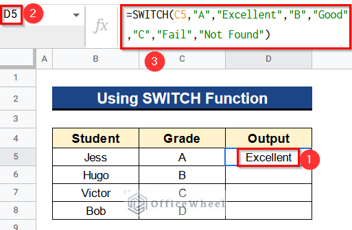
- Before all, put the following formula in Cell D5–
=SWITCH(C5,"A","Excellent","B","Good","C","Fail","Not Found")- Afterward, hit the Enter button to get the desired result.
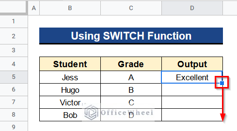
- Moreover, apply the Fill Handle tool to the rest of the cells of Column D.
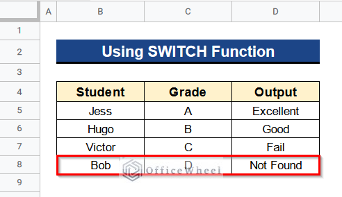
- In the end, you’ll see your desired comments in Column D. Additionally, you can find the comment “Not Found” in Row 8.
Conclusion
That’s all for now. Thank you for reading this article. In this article, I have discussed 5 useful fixes when the IFS function is returning a No Match Error (#N/A) in Google Sheets. Please comment in the comment section if you have any queries about this article. You will also find different articles related to google sheets on our officewheel.com. Visit the site and explore more.