In Google Sheets, you can classify data using the IF function. It determines whether or not a cell’s condition is true. If you want to combine many sets of criteria, you can use nested IF statements. Although nested IF statements are useful, they can produce very lengthy formulas that are challenging to deal with and can result in mistakes in your worksheet. Thankfully, you can utilize the IFS function, which is less complicated. In this article, I will show 3 simple examples of using the IFS function in Google Sheets.
What Is IFS Function in Google Sheets?
The IFS function in Google Sheets looks at several criteria and provides an output that matches to the first true condition.
Syntax
The syntax of the IFS function is as follows:
=IFS(condition1, value1, [condition2, value2, …])Arguments
The arguments of the IFS function are as follows:
| ARGUMENT | REQUIREMENT | FUNCTION |
|---|---|---|
| condition1 | Required | The initial condition is to be assessed. |
| value1 | Required | If condition1 is TRUE, this value is returned. |
| condition2, value2, … | Optional | If the initial condition is found to be false, additional conditions and values are assessed. |
Output
The formula IFS(A2 > 90, “A”, A2 > 80, “B”) will look for the value in Cell A2. If it is larger than 90, it returns A. If it is larger than 80, it returns B.
3 Ideal Examples of Using IFS Function in Google Sheets
Here, we will see 3 different examples of using the IFS function in Google Sheets. First, we will determine students’ performance based on their marks, then we will estimate total tax based on the tax rate on income, and after that, we will evaluate buyer parties’ choices based on multiple criteria using the IFS function in Google Sheets.
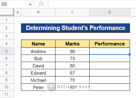
1. Determining Student’s Performance
Let’s imagine that we want to show how well students performed based on several aspects. If a student’s exam score is less than 70, their performance will be considered Bad. If a student scored greater than 70 but less than 80 on the test, they would be considered to have a Medium performance. Students who received exam scores more than or equal to 80 will be classified as Good performers.
Steps:
- Firstly, select the cell where you are going to apply the formula. In our case, we selected Cell D5.
- Next, type the formula below and press Enter–
=IFS(C5<70,"Bad",C5<80,"Medium",C5>=80,"Good")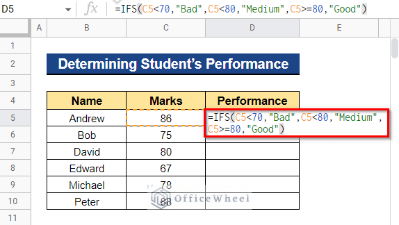
- It will display how well the student from Cell B5 performed on the exam. Now, drag the Fill Handle icon downward to apply the formula to the remaining cells.
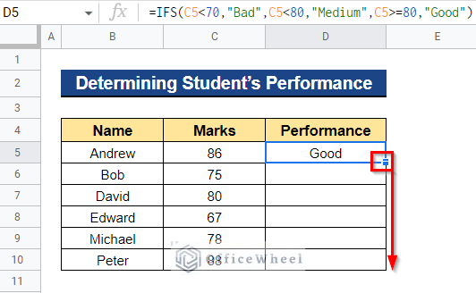
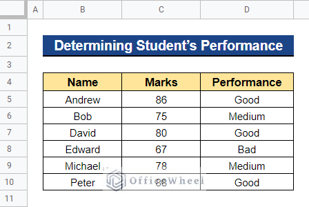
- Thus, it will display all of the student’s performance based on their marks on the exam.
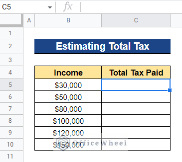
2. Estimating Total Tax
Assume we wish to calculate the total amount of tax paid depending on the income tax rate. We can do this using the IFS function. Below you’ll find a list of incomes, and for individuals making less than $50,000 per year, we have used a tax rate of 10%. People who earn more than $50,000 but less than $100,000 are required to pay a 20% tax. For people with incomes of more than $100,000, we have chosen a tax rate of 35%.
Steps:
- Select the cell to which you will be applying the formula first. In our instance, we decided on Cell C5.
- After that, enter the following formula and press Enter–
=IFS(B5<50000,0.1,B5<100000,0.2,B5>=100000,0.35)*B5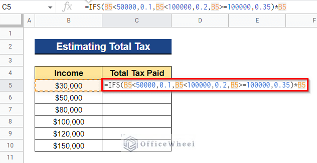
- It will show how much tax was paid on the income shown in Cell B5. To apply the formula to the remaining cells, now drag the Fill Handle symbol downward.
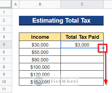
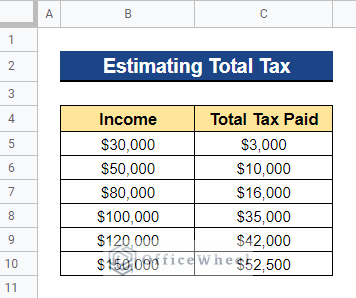
- As a result, depending on the income tax rate, it will show the entire amount of tax paid by the incomes listed in Column B.
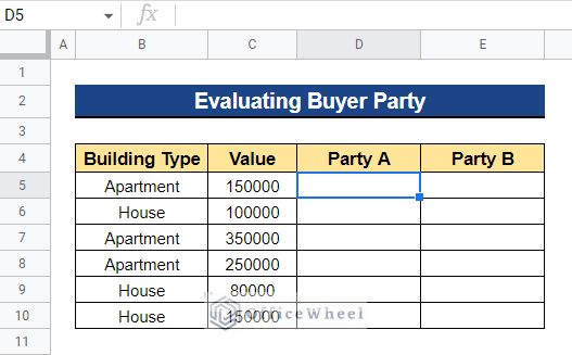
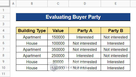
3. Evaluating Buyer Party
Consider the following scenario: two buyer groups have inspected potential houses. The agency wants to keep a record of everyone’s preferences. Combining the IFS, ISBLANK, and AND functions, we can accomplish this. Here, we will assume that Party A preferred apartments priced under $300k while Party B preferred houses over apartments.
Steps:
- Firstly, choose a cell to which you want to apply the formula. We chose Cell D5.
- Now, input the formula below and hit Enter–
=IFS(ISBLANK($C5)," ",AND(D$4="Party A",$B5="Apartment",$C5<300000),"Interested", AND(D$4="Party B", OR($B5="House")), "Interested",TRUE,"Not interested")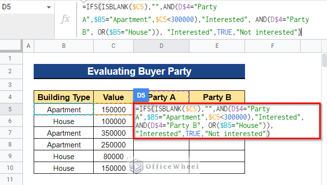
Formula Breakdown
- ISBLANK($C5)
First, it will determine whether Cell C5 is empty or not.
- AND(D$4=”Party A”,$B5=”Apartment”,$C5<300000)
If all of the parameters are logically true, the AND function returns true; if any of the parameters are logically untrue, it returns false.
- IFS(ISBLANK($C5),” “,AND(D$4=”Party A”,$B5=”Apartment”,$C5<300000),”Interested”, AND(D$4=”Party B”, OR($B5=”House”)), “Interested”,TRUE,”Not interested”)
The IFS function then examines multiple criteria and returns a value corresponding to the first true condition.
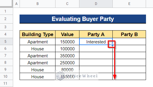
- For Party A, if the building type is Apartment and the Value of the Apartment is less than $300k, it will display Interested. Otherwise, it will display Not Interested. Now, to apply the formula to the remaining cells, drag the Fill Handle icon downward.
- Furthermore, to apply the formula for Party B also, drag the Fill Handle icon rightward.
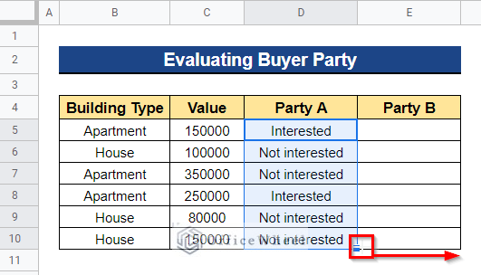
- Thus, it will display the two buyers’ preferences.
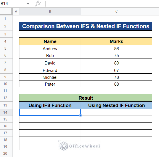
Comparison Between IFS Function and Nested IF Function in Google Sheets
You may test various parameters in a single formula using the IFS function in Google Sheets. However, if you need to test several conditions, the IF function may grow unwieldy, unsightly, and difficult to handle. In order to compare the IFS function and nested IF function, we will use the example of assessing students’ performance on an exam based on multiple conditions. A student’s performance will be considered Bad if their exam result is less than 70. A student would be judged to have a Medium performance if they received a test score of more than 70 but less than 80. Students who obtained exam scores more than or equal to 80 will be categorized as Good performers.
Steps:
- First, choose the cell to which you will be applying the formula. In this case, we chose Cell B14.
- Next, enter the following formula and press the Enter button-
=IFS(C5<70,"Bad",C5<80,"Medium",C5>=80,"Good")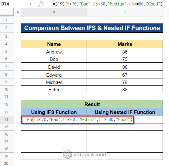
- It will show how well the student from Cell B5 performed on the test. Now, apply the formula to the remaining cells by dragging the Fill Handle icon downward.
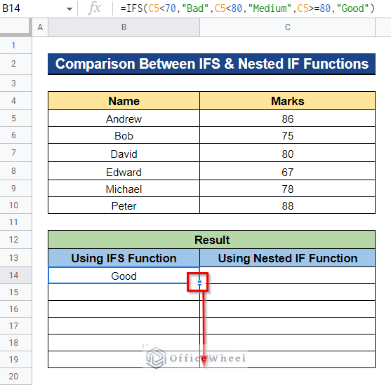
- As a result, depending on their exam scores, it will show all of the students’ performances. Now, to get a similar result using the IF function, first select the cell where you’ll apply the formula. We selected Cell C14.

- Next, enter the following formula and hit the Enter key-
=IF(C5<70,"Bad",IF(C5<80,"Medium",IF(C5>=80,"Good")))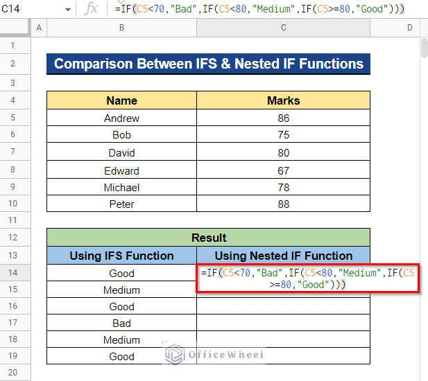
- To apply the formula to the remaining cells, now drag the Fill Handle symbol downward.
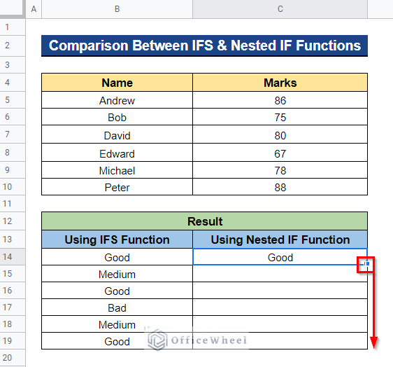
- Thus, it will display the desired output.
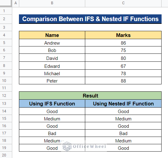
So, we have got a similar result using the IFS function and nested IF function and we observed that the IFS function is less complicated than the nested IF function.
Read More: How to Use IFS Between Two Numbers in Google Sheets
Conclusion
In this article, I have shown 3 simple examples of using the IFS function in Google Sheets. I have also shown a comparison between the IFS function and the nested IF function. I think this will be helpful. Please feel free to ask any quarries or suggest any ideas in the comment section below. To explore more, visit Officewheel.com.