Sometimes we need to differentiate outputs in the same dataset and every time doing it manually is quite complex and time-consuming. It would be much easier if we try conditional formatting to differentiate those conditions using if statement In this article, we will learn how to use if statement in conditional formatting in google sheets.
A Sample of Practice Spreadsheet
You may copy the spreadsheet below and practice by yourself.
How to Apply Conditional Formatting in Google Sheets
Conditional formatting highlight certain cell or range as per requirement. Here are the steps to apply conditional formatting below.
📌 Steps:
- First, select the range for applying conditional formatting.
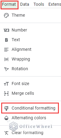
- Then click Format >> conditional formatting from the menu bar.
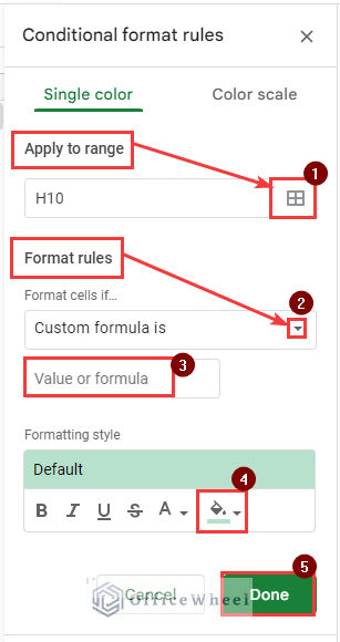
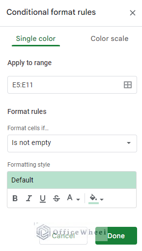
- After that, a conditional formatting window will pop up. Now modify “Apply to range”, “Format rules” and Formatting style as per the required condition and click Done.
2 Simple Examples of Using Google Sheets IF Statement in Conditional Formatting
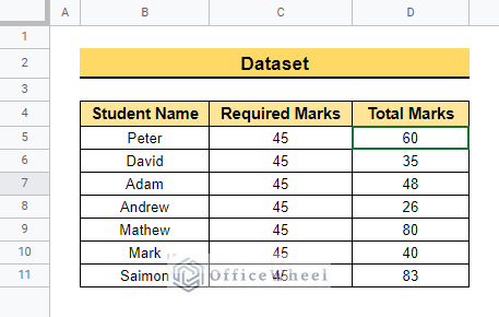
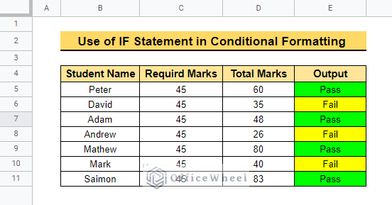
Here, the dataset below contains Student Name, Required Marks, and Total Marks. Here we will figure out who passed and who didn’t using the required marks and the total mark of a student. Now we will show how to use the if statement in conditional formatting in google sheets. So, Let’s Start.
1. Using Built-in IF Statement
Here, we will use the if statements in conditional formatting using the Text contains option in Format rules.
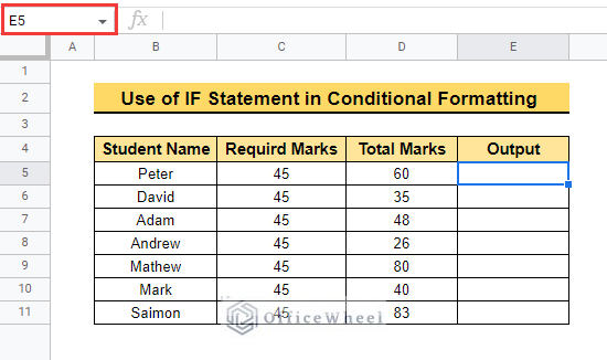
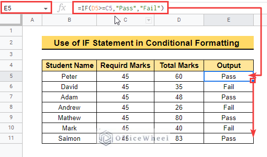
- First, Select cell E5 to enter the formula as below.
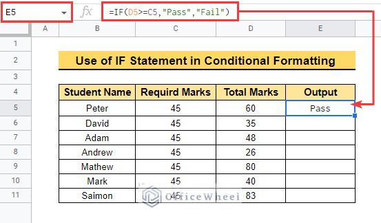
- Here, enter the IF function to determine which student passed as students will only pass if the total marks are more than the required marks.
=IF(D5>=C5,"Pass","Fail")- Now drag down the Fill Handle to copy the formula into the remaining cell of this dataset.
- After that, differentiate the output using conditional formatting.
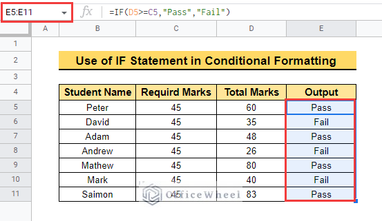
- First, select cell range E5:E11 to execute this method as below.
- Now, select Format >> Conditional formatting from the menu bar.
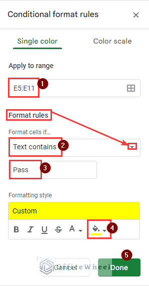
- Then, the “Conditional format rules” window will pop up which is required to be changed as below.
- After that, select “Text contains” from Format rules and type Pass into Value or formula box. Select a formatting color and click Done.
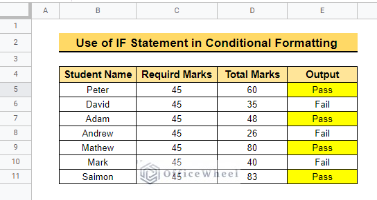
- Then, the output of applying condition for Pass is as below.
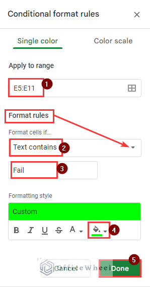
- Again apply conditional formatting for the text Fail.
- At last, the final output will be as below.
- Before applying conditional formatting change the color to differentiate two different conditions and click Done to execute the formula.
Similar Readings
- How to Use IF Function in Google Sheets (6 Suitable Examples)
- Highlight Cell If Value Exists in Another Column in Google Sheets
2. Applying Custom IF Statement
Here, we will use the if statement in conditional formatting using Custom Formula is in Format rules.
📌 Steps:
- First, complete the steps below and insert the IF function into the dataset.
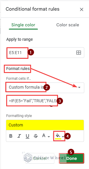
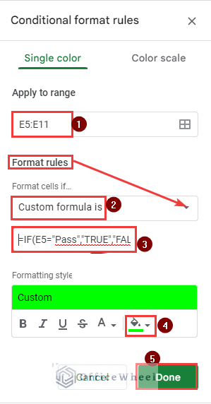
- Then select “Custom formula is” in the Formate rules box and enter the formula into the Value or formula Box as below any apply conditional formatting with the below changes.
=IF(E5="Fail","TRUE","FALSE")- Again repeat the process using another condition for formatting.
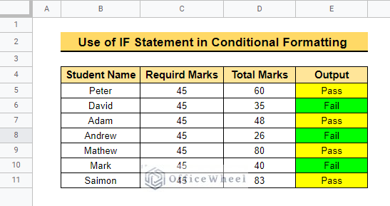
- Change the color from the Formatting style before clicking Done to differentiate the results.
=IF(E5="Pass","TRUE","FALSE")- At last, the final output is as below.
Read More: How to Use Nested IF Statements in Google Sheets (3 Examples)
Things to Remember
- Always try to differentiate with visible color while executing conditional formatting.
- Use the “Custom formula is” according to your preferences.
Conclusion
In this article, we explained how to apply conditional formatting and also explained how to use IF statement in conditional formatting in google sheets with some examples. Hopefully, the examples will help you to apply this method to your own dataset. Please let us know in the comment section if you have any further queries or suggestions. You may also visit our OfficeWheel blog to explore more Google Sheets-related articles.

