You can frequently search through data columns in a spreadsheet to identify a specific keyword. It is simple to perform this manually on smaller spreadsheets. Large spreadsheets make this task nearly impossible, though. Fortunately, Google Sheets comes with a number of built-in features that make it simple to search for data in your spreadsheets. Don’t worry; in this article, we’ll explain to you a few simple methods for searching in a column in Google Sheets.
3 Suitable Ways to Search in a Column in Google Sheets
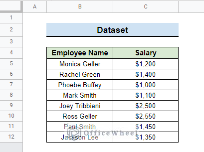
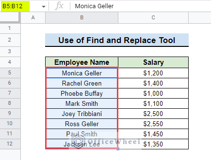
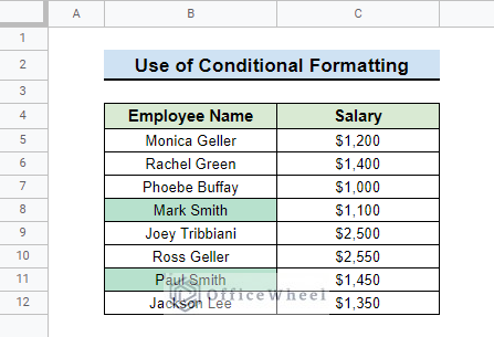
Assume you have a simplistic dataset with only two columns. Names of the employees are listed in the first column, and salaries are listed in the second. A sample of the dataset is shown here. Let us just say you want to search for a name in the employee name column. Here we will show you 3 simple ways to search in the Employee Name column in Google Sheets.
1. Use of Keyboard Shortcut
Using a Keyboard Shortcut in Google Sheets, you may quickly identify the cells that contain a given text string if your spreadsheet has cells with text. These are the few steps to do that.
📌 Steps:
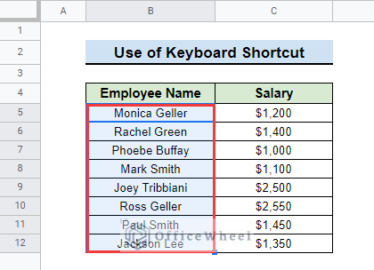
- First, open your Google Sheets and select the column in which you want to search your data. Here the selection range is B5:B12.
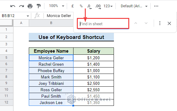
- Then, press CTRL + F on the keyboard and it will open a small Find in sheet box in the upper right corner of the Google Sheets window.
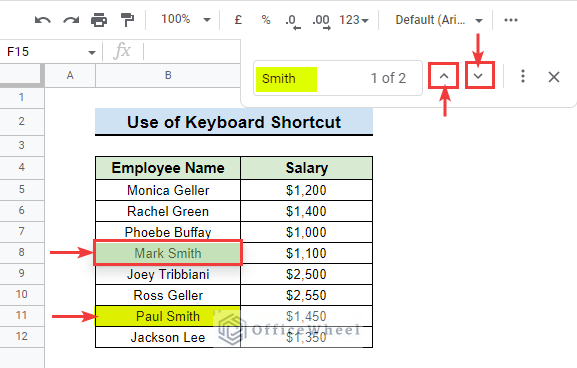
- Now, you need to type the text you want to search in a column in the popped-out box in the Google Sheets. Suppose you want to search for Smith. Then enter the keyword in the search box.
- After that, all the cells in the entire column containing that string will get highlighted. You can just explore them by clicking on the upward and downward arrows at the right side of the find box.
2. Utilize Find and Replace Tool
There is another built-in function in Google Sheets called the Find and Replace tool. It can be a handy way to search in a column in Google Spreadsheets. Let us say, we want to find the same name as earlier from the Employee Name column. The few steps to follow to do that are given below.
📌 Steps:
- Here, we want to find Smith. So select the column range from B5:B12 at first.
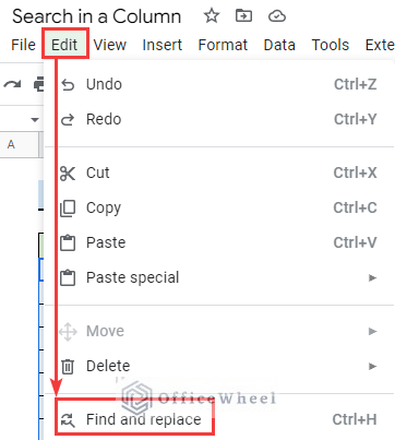
- Then, go to the Edit menu and select the Find and replace option.
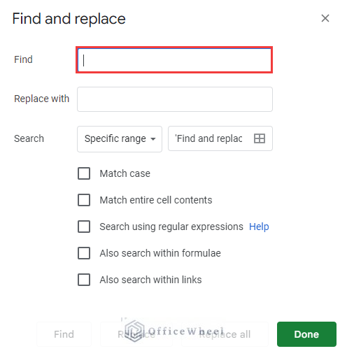
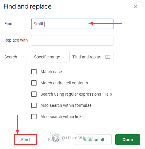
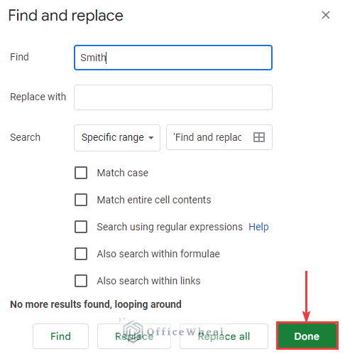
- After that, the Find and replace dialog box will appear. You can also do that by using the CTRL + H shortcut.
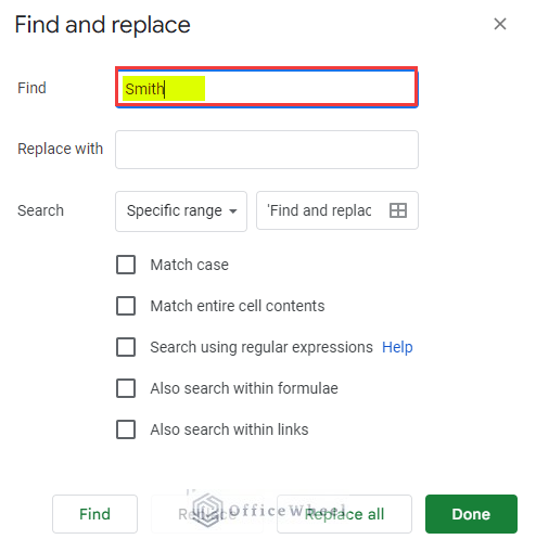
- Now, in the Find box, enter the text you want to search from the column. For example, we are looking for the word Smith. So we will type Smith in that box.
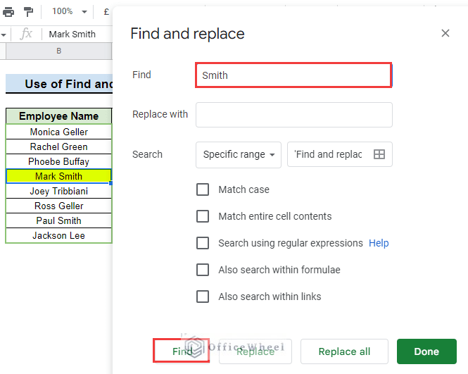
- Then press the Find button in the bottom left corner of the dialog box.
- This will highlight the first cell containing this text in the selected column.
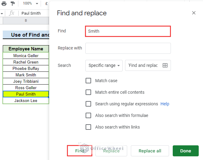
- Now, if there are more names related to the search keyword, you can press the Find button repeatedly to see the results.
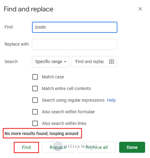
- Finally, when there is no more related word in the column after pressing the Find option, it will show you the notification “No more results found, looping around” just above the Find button.
- Now, you can finish your task by pressing the Done box at the bottom right corner of the dialog box.
Read More: How to Search and Replace in Google Sheets (2 Easy Ways)
3. Apply Conditional Formatting
The previous methods show results one by one. But you can apply conditional formatting if you want to find all the cells that contain the search keyword. So, here we will show you how to apply conditional formatting to search in a column in Google Sheets. To Search in a Column applying Conditional Formatting, there are two sub-methods.
3.1 Search in Single Column
You can search in a single column using conditional formatting. Follow the steps mentioned below to apply this approach.
📌 Steps:
- First, select the column from where you want to find the word. Here the range is B5:B12.
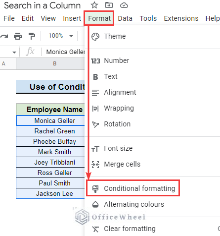
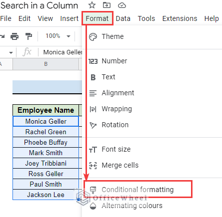
- Then, go to the Format tab in the ribbon and select the Conditional formatting option.
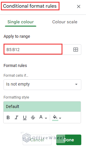
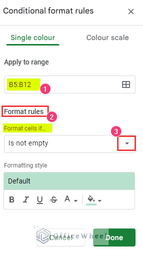
- After that, a new dialog box will appear on the right side of your Google Sheets window named Conditional format rules.
- In the popped-out window, you can see the selected range below the Apply to range option, that is showing the range we selected before.
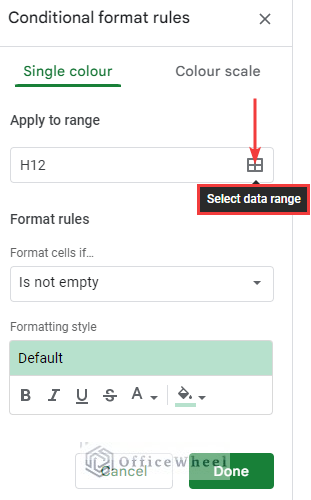
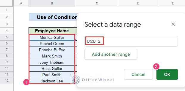
- If you forget to select the range then you can quickly type the range manually or click on the Select data range icon at the right.
- After that, the Select a data range dialog box will appear. Now select the range (B5:B12) in the dataset and press the OK button as shown below.
- After selecting the range, go to the Format rules option where Format cells if is showing and press the drop-down icon there.
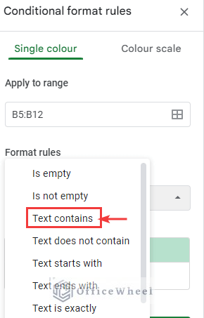
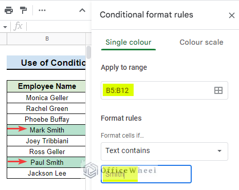
- Then, select Text Contains from the dropdown list as shown below.
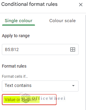
- Next, you will see a new Value or formula box below the drop-down list.
- Then, type the name you want to search in the selected column and you can see it will be highlighted in the column just like the image below.
- Finally, press the Done button to complete the task with Conditional Formatting.
Read More: How to Search for Text in Range in Google Sheets (4 Simple Ways)
3.2 Create a Search Box
In the earlier method, you need to remove the conditional formatting every time you want to search for a new keyword. You can create a search box using conditional formatting to fix this issue.
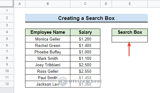
Suppose, we will use cell E5 as the search box.
📌 Steps:
- Then, go to the Format ribbon and click the Conditional Formatting option.
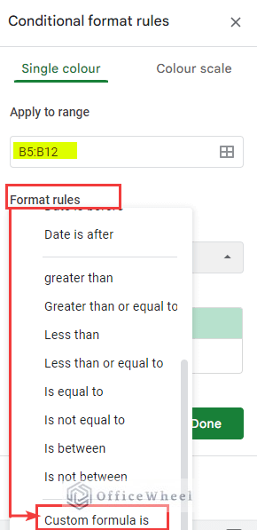
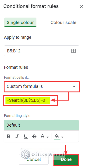
- After that, apply the range from B5:B12 in the Format Rules dialog box and choose the Custom Formula Is option.
- Then, apply the formula below the Custom formula is box and press Done after typing the formula correctly.
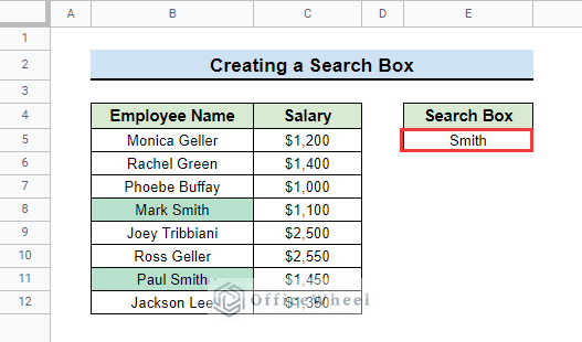
- Now type a name or part of the name of any employee in the search box. Then the matching results will be highlighted as follows.
Read More: How to Create a Search Box in Google Sheets (4 Easy Methods)
Things to Remember
- You can also replace any of the searched words in your Google Sheets using Find and Replace Tool.
- You have to select the Text Contains option in order to search in a column in Google Sheets.
Conclusion
In this article, we have covered 3 simple methods to search for a word in a column in Google Sheets to locate specific cells that contain the desired data. We hope it was helpful to you. If you know of any other methods please let us know through the comment section. For more techniques and strategies related to working in Google Sheets, you can explore our OfficeWheel website.

