The human eye is not particularly good at detecting minute variations or similarities between data objects when working with vast volumes of data. Fortunately, data processing tools like Google Sheets can notice minutiae that even the most skilled human eye could overlook. Therefore, actions like comparing columns, identifying discrepancies, and highlighting similarities are completed quickly, accurately, and effortlessly. In this article, I will demonstrate 6 simple methods of comparing and finding match cells between two columns in Google Sheets.
6 Ideal Methods to Match Cells Between Two Columns in Google Sheets
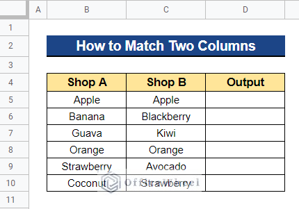
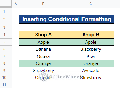
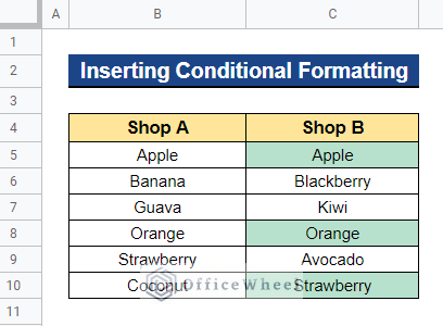
We will use the dataset below to demonstrate the examples of comparing and finding match cells between two columns in Google Sheets. The dataset contains product details of two different shops. Now we will use 6 different techniques to find matches between these two columns in Google Sheets.
1. Using Equal Operator
This technique allows us to search Google Sheets for a complete row match between two columns by row. It is one of the quickest methods for locating row matches.
Steps:
- First, select a cell where you want to apply the formula. In our case, we selected Cell D5. Now, type the formula below and press Enter–
=B5=C5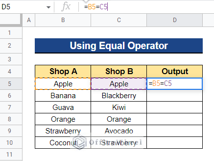
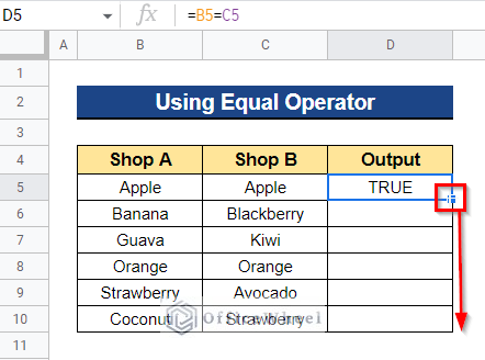
- It will return TRUE if the cells in the row match, and FALSE Now drag the Fill Handle icon downward to apply the formula to the remaining cells.
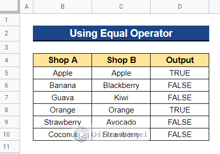
- Therefore, it will return TRUE if the row of these two columns matches, otherwise FALSE.
2. Applying IF Function
Using the IF function is another method for searching Google Sheets for a complete row match between two columns. Additionally, it is one of the easiest ways to find row matches. The main advantage is that you may pick what to display if the row of these two columns matches.
Steps:
- First, choose the cell to which you wish to apply the formula. In our situation, we chose Cell D5. Enter the following formula and hit Enter–
=IF(B5=C5,"Match","Different")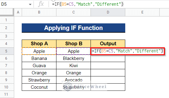
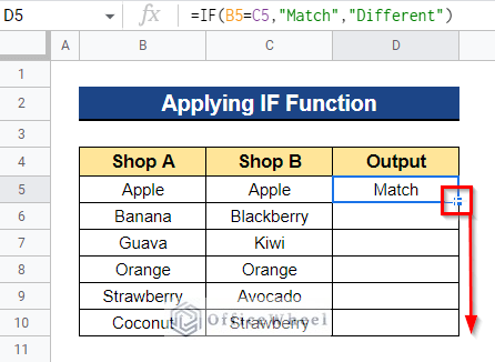
- If the cells in the row match, it will return Match; if not, it will return Different. To apply the formula to the remaining cells, now drag the Fill Handle symbol downward.
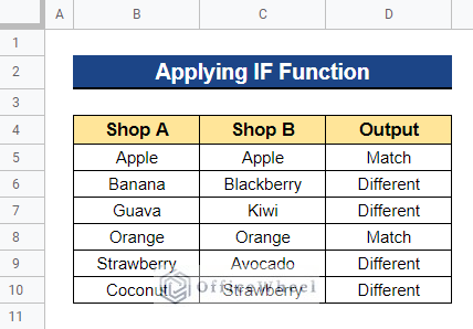
- As a result, it will return Match if the rows of these two columns match and Different otherwise.
Read More: How to Return Exact Match in Google Sheets (7 Suitable Ways)
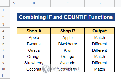
3. Combining IF and COUNTIF Functions
In Google Sheets, we might occasionally wish to look for matching data instead of row duplicates across two columns. To achieve this, we may combine the IF and COUNTIF functions.
Steps:
- Choose the cell to which you wish to apply the formula first. We chose Cell D5. Now, enter the following formula and press the Enter button-
=IF(COUNTIF(B$5:B$10,C5)=0,"Different","Match")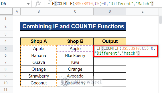
Formula Breakdown
- COUNTIF(B$5:B$10,C5)
The COUNTIF function will first count how many times Cell C5 appears within the range of Cells B5:B10.
- IF(COUNTIF(B$5:B$10,C5)=0,”Different”,”Match”)
If no matches are discovered, the IF function will then return Different; otherwise, it will return Match.
- If the text in Cell C5 is present in Column B, it will return Match; otherwise, it will return Different. To apply the formula to the remaining cells, drag the Fill Handle symbol downward.

- As a result, it will return Match if there are duplicate quantities across the two columns and Different otherwise.
4. Employing VLOOKUP Function
Using the VLOOKUP function in Google Sheets is an alternative method to search for matching data rather than row duplicates across two columns. Using this approach, we can identify duplicates between the two columns.
Steps:
- First, decide which cell you want the formula to be applied to. We selected Cell D5. Now, input the formula below and press Enter–
=VLOOKUP(C5, $B$5:$B$10, 1, FALSE)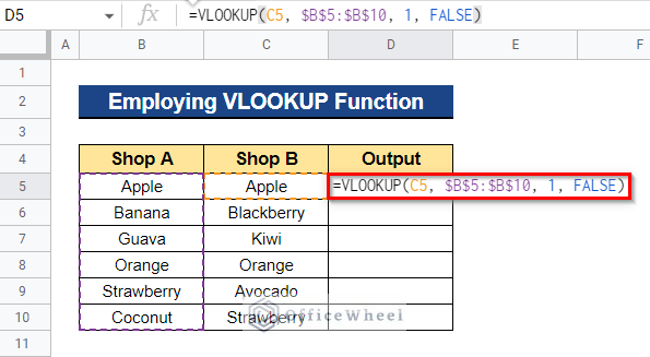
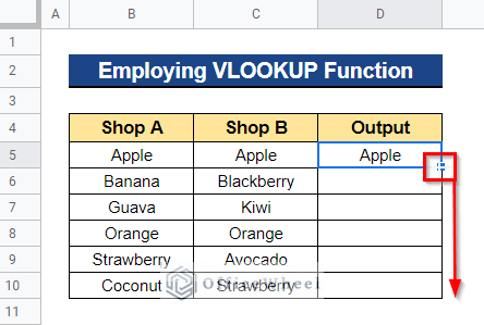
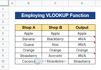
- It will search Cell C5 through Column B for the text, and if it is found, it will return that text. Otherwise, a red error notice will appear. Now, to apply the formula to the remaining cells, drag the Fill Handle symbol downward.
- As a result, a red error warning is displayed next to each unique value in Column C, and duplicate text is displayed next to each duplicate value.
5. Merging INDEX and MATCH Functions
Instead of looking for row duplication across two columns, another way to find matching data between two columns in Google Sheets is to combine the INDEX and MATCH functions. This method allows us to spot duplication between the two columns. This approach is comparable to the VLOOKUP approach.
Steps:
- Pick the cell to which you want to apply the formula first. We selected Cell D5. Now input the formula below and press the Enter button-
=INDEX(B$5:B$10,MATCH(C5,B$5:B$10,0))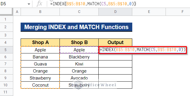
Formula Breakdown
- MATCH(C5,B$5:B$10,0)
First, the MATCH function returns the position of Cell C5 in a range of Cell B5:B10.
- INDEX(B$5:B$10,MATCH(C5,B$5:B$10,0))
Then the INDEX function will give back the content of a cell, defined by the column and row offset.
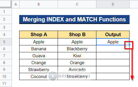
- Cell C5 through Column B will be searched, and if the text is found, it will be shown. If not, a red error notice will appear. Now apply the formula to the remaining cells by dragging the Fill Handle icon downward.
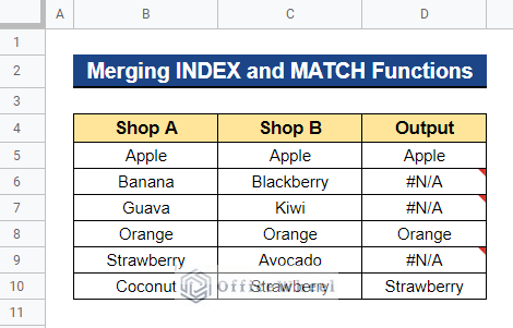
- As a consequence, the duplicate text is displayed in Column D next to each duplicate value in Column C and a red error notice is presented in Column D next to each unique value in Column C.
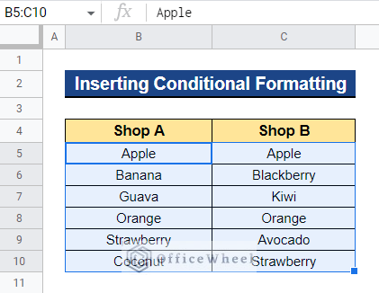
6. Inserting Conditional Formatting
In Google Sheets, Conditional Formatting may be added to discover matches between two columns. To make the datasheet easier to visualize, we can locate matches and highlight those matches. Utilizing the Conditional Formatting rule, we may locate and highlight a complete row match or identify duplicates between two columns.
6.1 For Row Match
Using conditional formatting, we can find and highlight a complete row match between two columns. To achieve this, we’ll use the equal operator.
Steps:
- First, select the entire dataset to which you will apply the conditional formatting rules. We selected Cell B5:C10.
- Now, go to the Format menu from the top menu bar and select Conditional formatting.
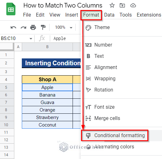
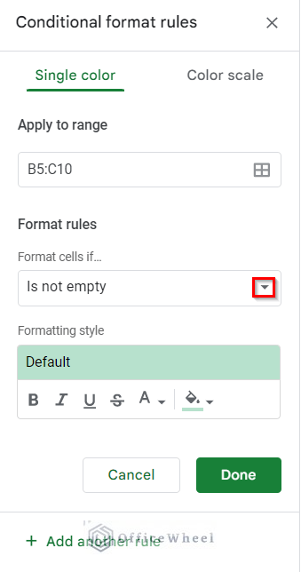
- As a result, a Conditional format rules dialog box will appear. Now click on the drop-down icon from the Format cells if… option.
- Then, select Custom formula is from the Format cells if… In the Values section, enter the formula below. It will detect the complete row match. You may choose any color to highlight those row matches from the color icon in the Formatting style.
=$B5=$C5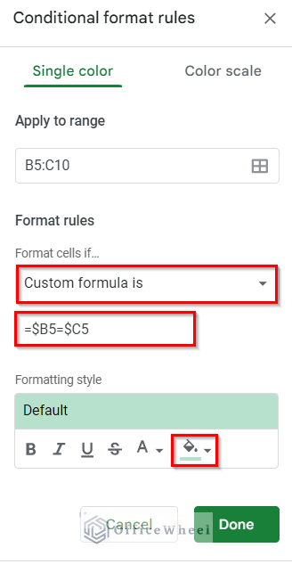
- Thus, it will highlight all the complete row matches between two columns.
6.2 For Entire Column
We may locate and identify duplication between two columns by using conditional formatting. We’ll make use of the COUNTIF function to do this.
Steps:
- Choose the second column to which you will apply the conditional formatting rules first. We chose Cell C5:C10. Select Conditional formatting from the Format menu in the top menu bar now.
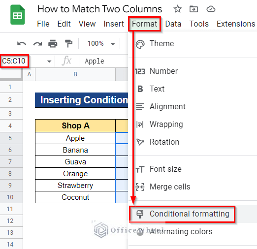
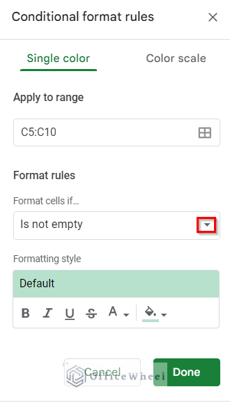
- A Conditional format rules dialog box will therefore show up. Click on the Format cells if… drop-down icon to continue.
- Then, from the Format cells if… option, choose Custom formula is. Enter the following formula in the Values It will identify the duplicates in Column C. From the color icon in the Formatting style, you may select any color to highlight those duplicates.
=COUNTIF($B$5:$B$10,C5)>0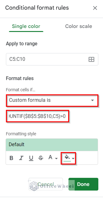
- Thus, it will highlight all the duplicates in Column C.
Conclusion
In this article, I have shown 6 simple examples of comparing and finding match cells between two columns in Google Sheets. I have shown how to get a complete row match as well as all the duplicates between two columns. I hope this will be helpful. Please feel free to ask any quarries and comment on any ideas in the comment section below. Visit Officewheel.com to explore more.