Since slicers are essentially a type of filter, there can arise situations where the user might need to customize the filter conditions to suit their or their organization’s needs. And much like filters, slicers in Google Sheets allow users to input a custom formula into them.
In this article, we will look at how we can use custom formulas in a Google Sheets slicer with a few distinct examples.
Let’s get started.
A Few Quick Notes About Google Sheets Slicers
Google Sheets slicers are a quick and easy way to filter data in a worksheet. It has a few situational advantages over filters and is a great way to customize dashboards.
Thus, we have a few points to keep in mind when using slicers in Google Sheets:
- A slicer can only work with a single column at a time.
- You can add multiple conditions using a slicer by adding more slicers to the worksheet.
- When adding multiple slicers, make sure to have the same source data range.
- A Google Sheets slicer filter affects all entities that use the same source data range. That includes pivot tables and charts.
- Formulas that use the same data range are unaffected by slicers.
- A filter produced by a slicer can be saved as a default filter template.
Using a Custom Formula in a Google Sheets Slicer
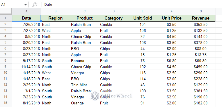
For this article, we will use the following worksheet as our data source:
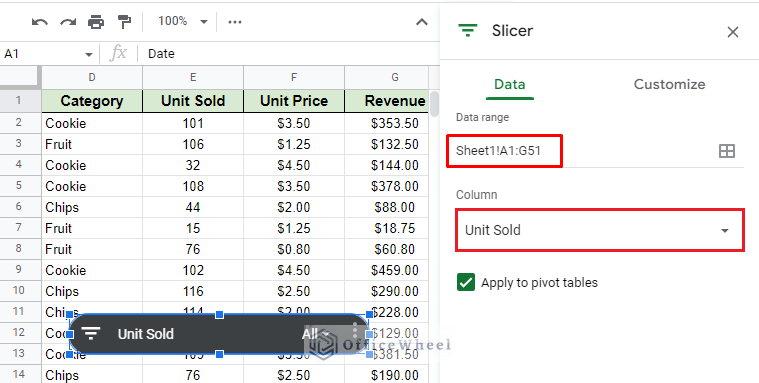
For simplicity’s sake, we have inserted a simple slicer for the range of the current dataset. The column condition is for ‘Unit Sold’ which we will use to add custom filters to.
Learn More about adding and using slicers: Google Sheets Slicer Tutorial
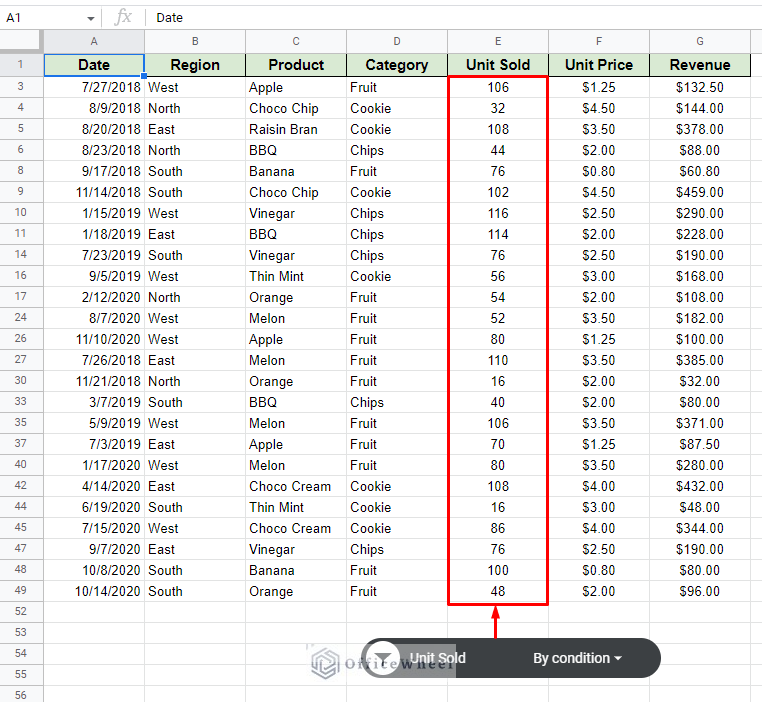
In this example, we will try to filter all the numbers of units sold by even numbers.
Naturally, this condition is not available by default in the ‘Filter by conditions’ menu; thus, we must use a Custom Formula.
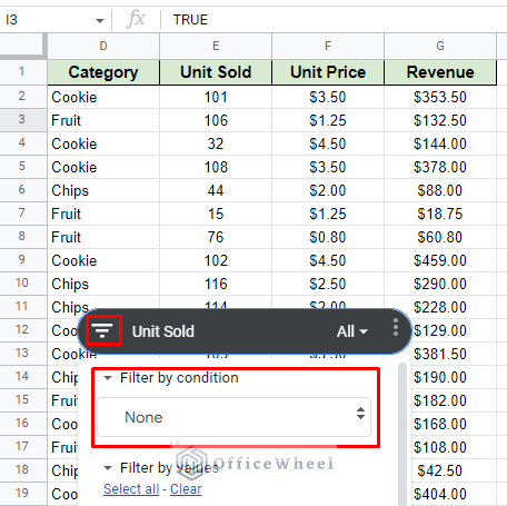
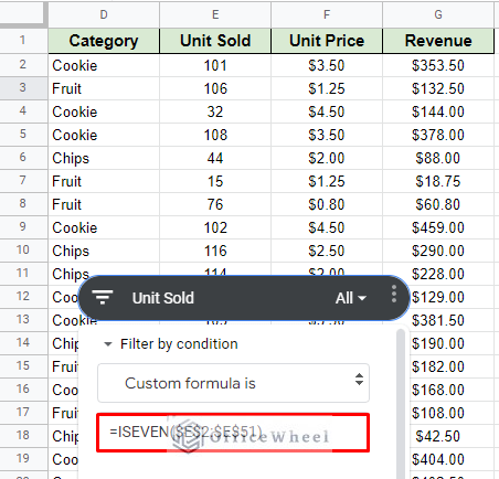
Step 1: Click on the filter icon of the slicer to bring out the filter menu. Here, open the ‘Filter by condition’ option.
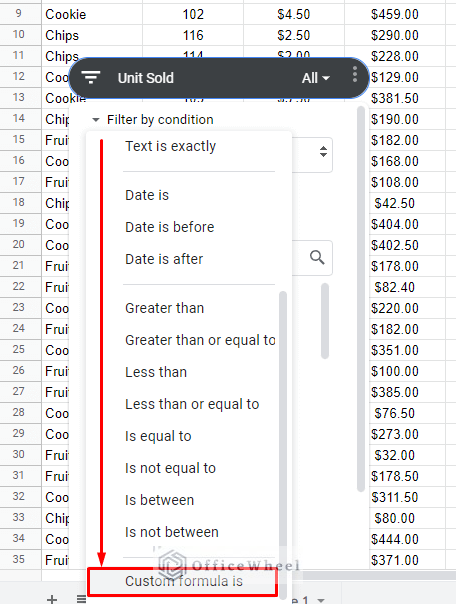
Step 2: From the drop-down, scroll to the bottom to find the ‘Custom formula is’ option.
Step 3: A new formula field will appear. Enter the following formula to filter only the even number of units sold:
=ISEVEN($E$2:$E$51)Step 4: Click OK to see the filter result.
With the basics now out of the way, let’s look at something more practical.
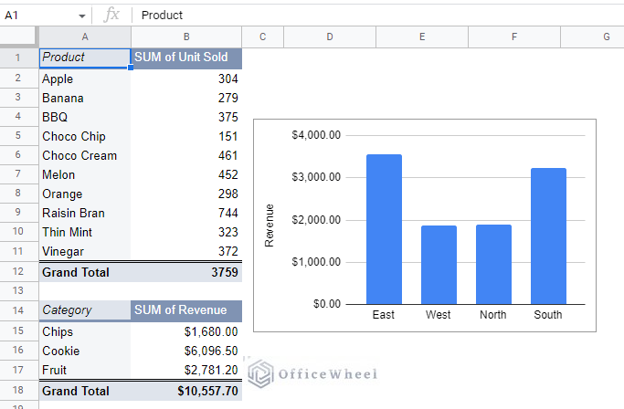
Here, we have a simple dashboard containing a couple of pivot tables and a corresponding chart.
The Google Sheets slicer truly shines working alongside pivot tables and dashboards. And we have two examples for you where we use the capabilities of using a custom formula in a Google Sheets slicer.
Example 1: Filter Results According to Weekdays Using a Google Sheets Slicer
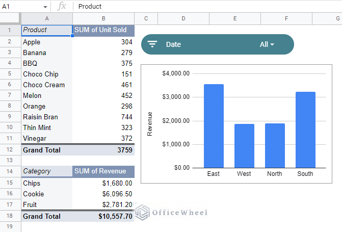
In this example, we will add and use a slicer based on the Date column:
Learn more about slicers in pivot tables: Apply a Pivot Table Slicer in Google Sheets (An Easy Guide)
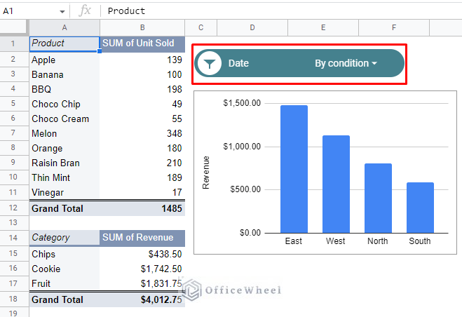
Using this slicer, we will try to find all the data for the current dashboard for dates that are Thursdays and Fridays.
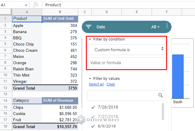
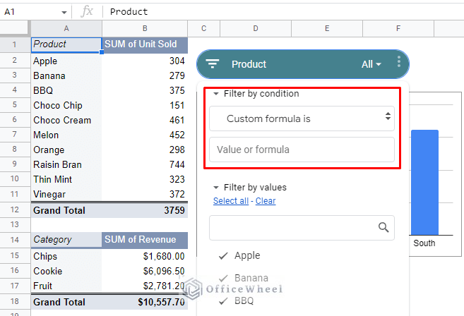
Step 1: Set the slicer to ‘Filter by condition’ and ‘Custom formula is’.
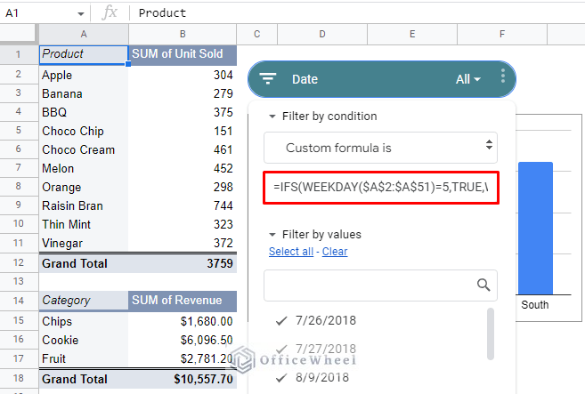
Step 2: Input the following formula:
IFS(WEEKDAY($A$2:$A$51)=5,TRUE,WEEKDAY($A$2:$A$51)=6,TRUE,WEEKDAY($A$2:$A$51)<5,FALSE)The WEEKDAY function takes a date (column A of the data range) and returns the corresponding weekday number. For Thursday and Friday, it is 5 and 6 respectively.
Using the IFS function allows us to set a Boolean condition to return a TRUE value when a date falls on a Thursday or Friday. Otherwise, it returns FALSE.
Step 3: Click OK to apply the formula.
Example 2: Filter Partial Text Match Using a Slicer
Perhaps one of the most useful filters in a spreadsheet is the partial match filter.
As usual, the best way to approach a partial text match formula is by using REGEXMATCH. The formula stems from the use of regular expressions.
For this example, we will filter all the Products that start with the keyword ‘Choco’.
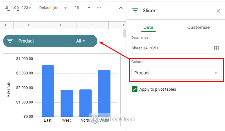
Step 1: Insert a new slicer or update the existing one to follow the column Product.
Step 2: Set the slicer to ‘Filter by condition’. Select the drip-down and set it to ‘Custom formula is’.
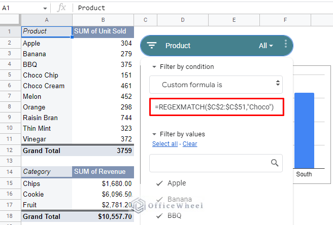
Step 3: Input the following formula:
=REGEXMATCH($C$2:$C$51,"Choco")The REGEXMATCH goes through the given range and returns TRUE if a match is found. Otherwise, it is FALSE and ignored.
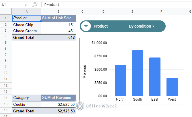
Step 4: Click OK to see the results.
The slicer custom formula has correctly recognized the partial matches. Formulas like these are best used when you have a match through a lot of unique values.
Final Words
Adding a custom formula to a Google Sheets slicer opens up a new dimension to how we can customize and present a dashboard or just pivot tables.
Feel free to leave any queries or advice you might have for us in the comments section below.

