We often use the HYPERLINK function for creating a shortcut to another location in the current workbook or opening any document stored on a network server or the Internet. In this article, we’ll demonstrate a step-by-step procedure for how you can hyperlink data to another sheet with the dynamic HYPERLINK formula in Google Sheets. Also, I’ll show you two alternatives to applying the formula.
A Sample of Practice Spreadsheet
You can copy our practice spreadsheets by clicking on the following link. The spreadsheet contains an overview of the datasheet and an outline of the described ways to hyperlink data to another sheet in Google Sheets.
Step-by-Step Procedure to Hyperlink Data to Another Sheet with Formula in Google Sheets
Here, we’ll use the HYPERLINK function to create a shortcut to another sheet. Follow the steps below to create and execute the hyperlink.
Step 1: Prepare Dataset for Two Sheets
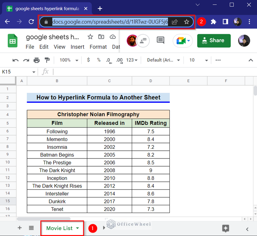
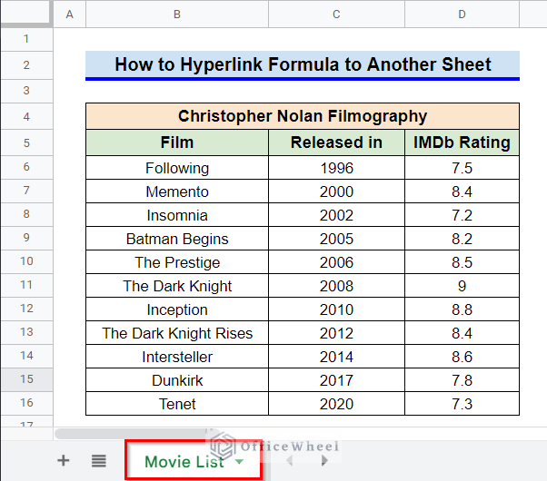
- First, let’s create a dataset like the following in a worksheet titled “Movie List” in Google Sheets. We’ll create a shortcut using the HYPERLINK function that jumps to this worksheet.

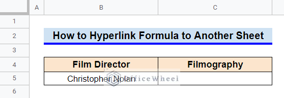
- In another worksheet, create another dataset like the following. We’ll create the hyperlink in this table.
Step 2: Copy Sheet Link
- In this step, we have to copy the link of the sheet where we want the link to jump over. For that, open the “Movie List” worksheet and copy the site link by selecting it first and then using the keyboard shortcut CTRL+C.
Step 3: Insert Dynamic Hyperlink Formula
- Now, go to the sheet where you want to create the hyperlink.
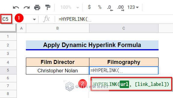
- First, select the cell where you want to create the hyperlink (i.e. Cell C5).
- To create the HYPERLINK formula, we require two arguments: the URL (the link we copied), and the link label.
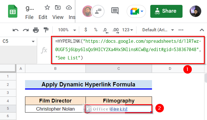
- In the HYPERLINK formula, paste the copied link within a double quote symbol (“”) as the URL and enter “See List” as the link label. The formula should look like this:
=HYPERLINK("https://docs.google.com/spreadsheets/d/1lRTwz-0UGF5j6Upy6lsQo9HICY2Xa4HxSNlinsKCwBg/edit#gid=538367048", "See List")- Finally, press Enter key to see the output.
Step 4: Final Output
- To see the hyperlink, hover your mouse pointer over the hyperlinked cell. Click on the popped-up link to jump to the linked sheet.
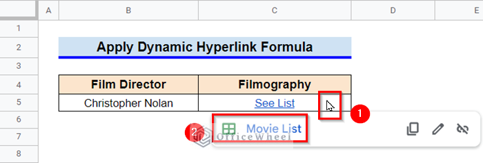
- As soon as you click on the link, you will jump to the “Movie List” worksheet.
Read More: How to Get Hyperlink from Cell in Google Sheets (4 Quick Tricks)
How to Hyperlink Data to Another Sheet Without Formula in Google Sheets
Can we apply a hyperlink from one sheet to another without using a formula? The answer is a resounding Yes! In this section, I’ll show you two alternative ways to formula for hyperlinking data to another sheet in Google Sheets.
1. Using Insert Link Command with URL
You can insert URL of the worksheet using Insert Link command that can be selected from the Insert ribbon or right-click of mouse.
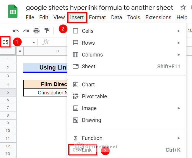
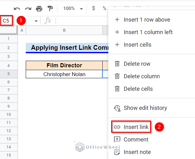
- First, select Cell C5 and then go to the Insert ribbon and select Link command from there.
- A window like the following will pop up below Cell C5.
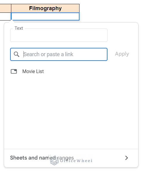
- Another way to open a pop-up window like the preceding image is to select Cell C5 and then click on the right button of your mouse and from the pop-up commands, select the Insert Link command.
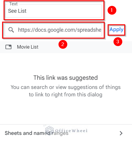
- Now, set the Text as “See List” and paste the copied link using the keyboard shortcut CTRL+V in the search box. After that, click on Apply.
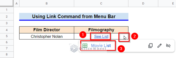
- A hyperlink has been created in the required cell. Hover your mouse pointer over the cell to see the link of the sheet you want to jump to.
Read More: How to Extract URL from Hyperlink in Google Sheets (3 Ways)
2. Using Insert Link Command with Sheet Name and Range
You can also create a hyperlink without copying the URL by entering the sheet name.
Steps:
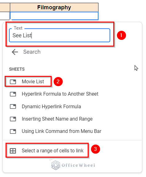
- Follow the first three steps from the previous method to open a window like the following and click on Sheet and Named Ranges from there.
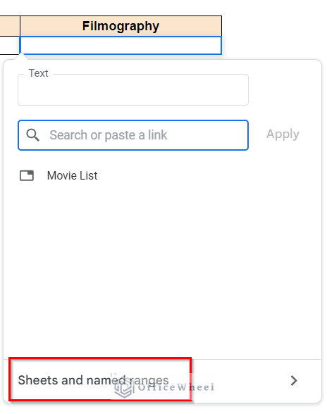
- Set the Text as “See List” and click on the name of the sheet (i.e. Movie List). You can also choose a specific cell range by selecting the Select a Range of Cells to Link option.
- A hyperlink has been created in the required cell. Hover your mouse pointer over the cell to see the link of the sheet you want to jump to.
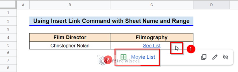
- Click on the link to jump to the linked sheet.
Read More:
Things to Be Considered
- Remember to put the URL in a double quote symbol (“”) while using the HYPERLINK function.
Conclusion
This concludes our article on how to Hyperlink data to another sheet with formula in Google Sheets. I hope the demonstrated steps were sufficient for your requirements. Feel free to leave your thoughts on the article in the comment box. Visit our website OfficeWheel.com for more helpful articles.