Everything is online-based these days. We frequently need to link web pages, publications, and even Google Sheets or Tables—not just for quick access, but also for reliable reference. The HYPERLINK function in Google Sheets makes this functionality easily accessible. You may learn how to make the most of this function with the help of this article.
A Sample of Practice Spreadsheet
You can copy the spreadsheet that we’ve used to prepare this article.
What Is HYPERLINK Function in Google Sheets?
A hyperlink enables easy access to a system file or folder as well as an external website. A lot of websites utilize them to link to other websites. The HYPERLINK function in Google Sheets is helpful for creating hyperlinks within cells.
Syntax
The HYPERLINK function has the following syntax.
HYPERLINK(URL, [link_label])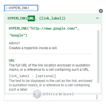
Argument
The HYPERLINK function has the following arguments.
| Argument | Requirement | Function |
|---|---|---|
| URL | Required | The full URL of the link location or a reference to a cell. |
| [link_label] | Optional | The text is to be displayed as the link in the cell. It is by default the URL. |
Output
The formula =HYPERLINK(“https://www.google.com/”,”Google”), for example, will make the word Google hyperlinked to the web address: https://www.google.com/.
2 Simple Ways to Use the HYPERLINK Function in Google Sheets
It’s not easy to add links using the Google Sheets HYPERLINK function. However, we could perhaps easily use this method depending on our needs and database. For clarification, go through the examples.
1. General Application
In Google Sheets, there are primarily two ways to use the HYPERLINK function. To illustrate each use, we will use a straightforward example.
1.1 Using Full Web Address
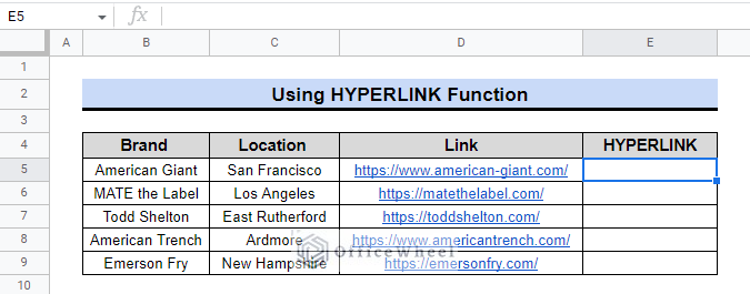
Assume we have information about the top clothing brands in the USA. We wish to make their official website instantly accessible from the data table. To make the functionality practical, we’ll take the next few steps.
Steps:
- We’ll start by choosing cell E5.
- Second, we’ll use “=” to type the function name. In this instance,
=HYPERLINK(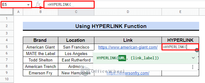
- We must place the URL inside quotation marks after the first set of parentheses.
=HYPERLINK("https://www.american-giant.com/"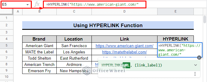
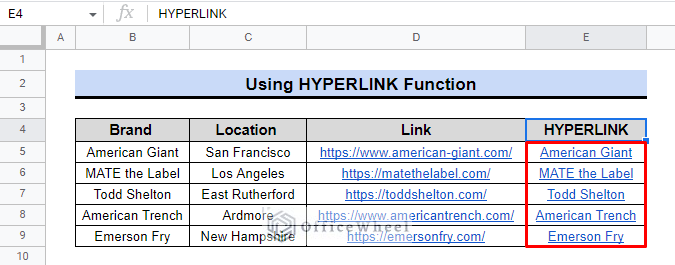
- Following that, we will use the brand name as the link label for the URL. It is American Giant in this case.
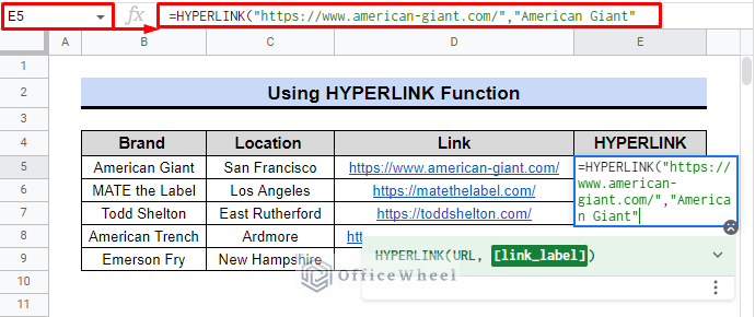
- Either press ENTER or close the parentheses. Final formula:
=HYPERLINK("https://www.american-giant.com/","American Giant")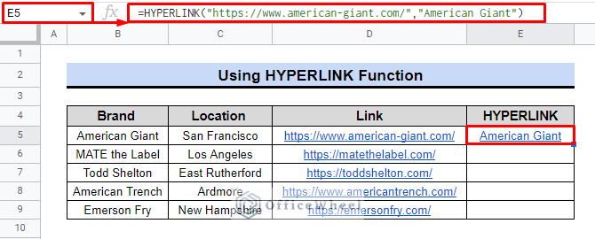
The word American Giant is now underlined and shown as a hyperlink, as can be seen in the image above.
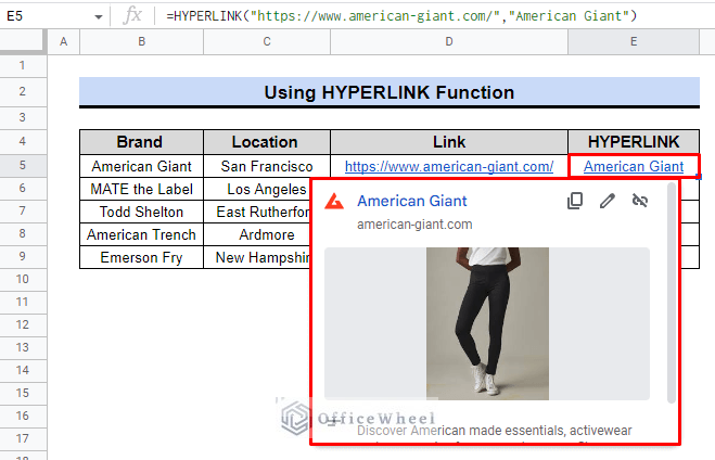
The link with its cover image and meta description will now appear automatically if we select cell E5.
Read More: How to Extract URL from Hyperlink in Google Sheets (3 Ways)
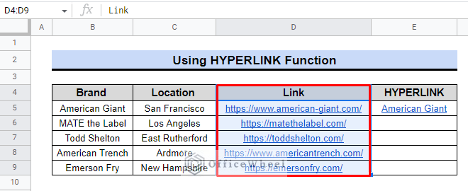
1.2 Utilizing Cell Reference
We can simply use the cells to generate a hyperlink because the table already contains the “Link” column. To understand the concept, go over the next few steps.
Step:
- Select cell E6 first.
- To generate a hyperlink, we’ll use the formula below.
=HYPERLINK(D6,B6)- Here, D6 serves as a URL reference and the label for the link is B6.
- Press ENTER once again to reveal the outcome.
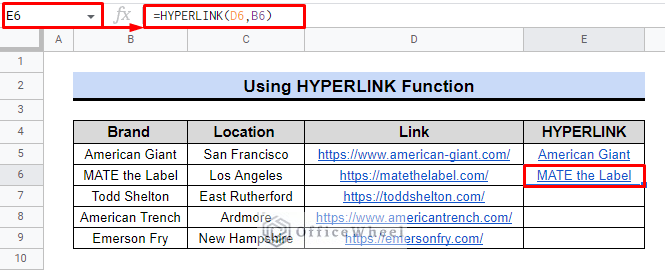
As you can see in the image, we can also generate hyperlinks by using cell values in the equation.
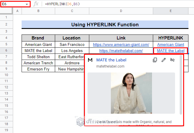
When we clicked on the cell in this instance as well, a similar preview window popped with the link.
Read More: How to Get Hyperlink from Cell in Google Sheets (4 Quick Tricks)
2. Advanced Application
This function allows us to link or connect any cells, tables, or data within the spreadsheet. Within the spreadsheet, there are two scenarios. We’ll discuss each scenario with a roughly equivalent example.
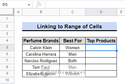
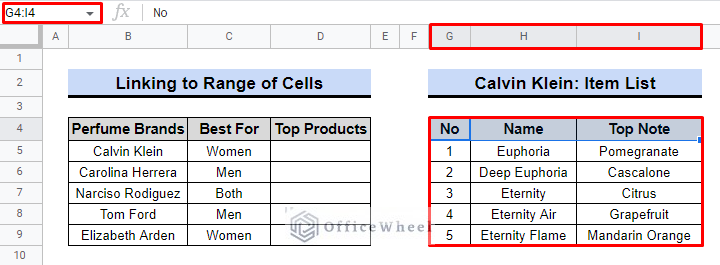
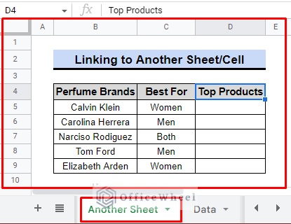
Take into account that we have data on the leading perfume brands in the USA. In addition, we have information on the best products from each company. They are, however, on a different page or table. In the table, we wish to connect all of them.
2.1 Connecting to a Cell or Range of Cells
The HYPERLINK function allows us to link a single cell or a range of cells within the spreadsheet. Unlike the last procedure, we must first construct a dummy hyperlink. We will then be able to link the cell, a range of cells, or the sheet. Check out the steps below.
Steps:
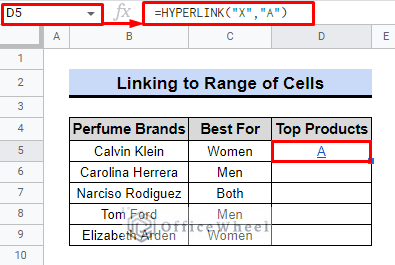
- Select the cell to D5 begin.
- To generate the dummy hyperlink, we’ll use the formula below.
=HYPERLINK("X","A")- In this case, X act as the URL and A is the label of the URL.
- To complete, press ENTER.
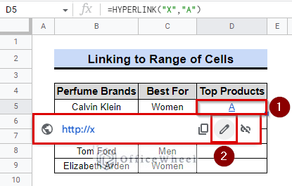
- After that, clicking the link will cause a little window with a white background to emerge.
- To open the edit menu, select the Edit link option.
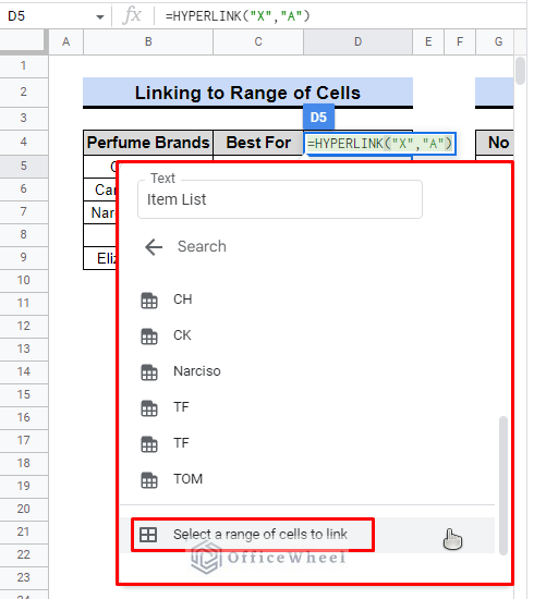
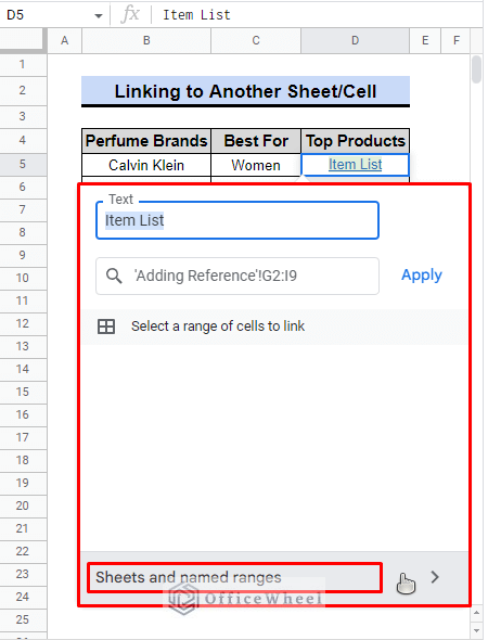
- We will first modify the label in the new window using the Text bar.
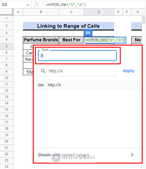
- Instead of “A“, we will type “Item List” as the link label in the text box.
- After that, select “Sheet and named ranges.” It will lead us to a fresh array of information.

- We’ll find “Select a range of cells to link” at the bottom of the window. Click it.
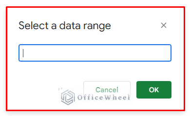
- A new window titled “Select data range” will appear.
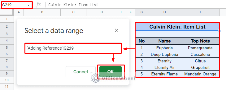
- We’ll choose the G2 through I9 cell range.
- To finish, click OK.
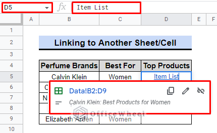
Now we’ll get the same result as seen in the image.
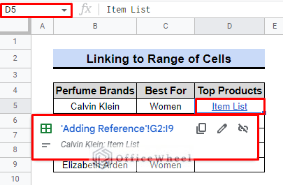
The reference table will be immediately accessible to us if we click the following link.
Read More: How to Hyperlink Data to Another Sheet with Formula in Google Sheets
2.2 Linking Another Sheet
Assume that another page contains the data for the top product item. Using the procedures from before, we can also incorporate it. However, we can apply some tricks to speed up the process. Check out the steps listed below.
Steps:
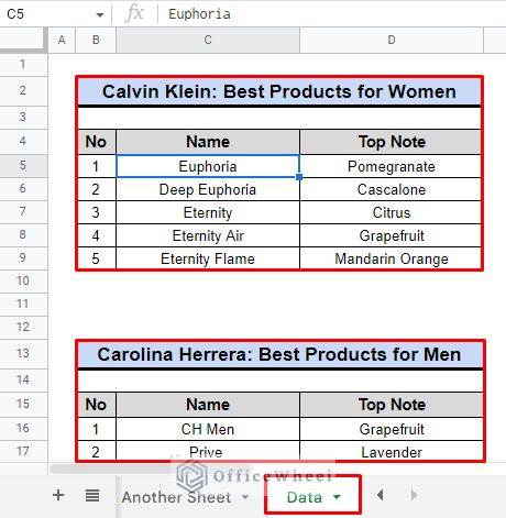
- We will start by looking at the Data sheet from Another sheet. The product lists are all there, organized by brand.
- We will now select the cells from B2 to D9 here.
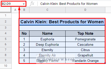
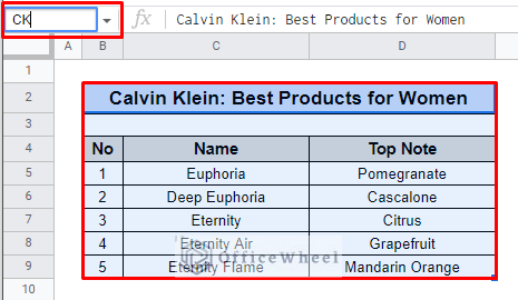
- Give them a name in the name box from the upper left corner. such as CK in this instance.
- What we’ve just created is called a named range.
- We will now return to the Top Products column. To access the Edit menu, select cell D5.
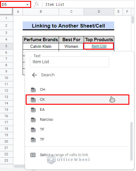
- We’ll choose the Sheets and named ranges option once more.
- A list of the table names will be available. One of them is CK.
- To finish this work, click CK.
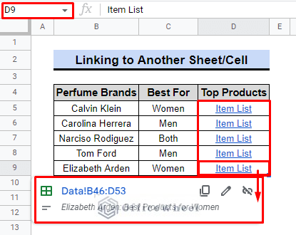
- After then, we shall see a picture similar to the one below. If we select the cell, it will give a preview of the data source. In this situation, DATA!B2:D9.
Now that the cells are connected, clicking one of them will send us directly to the item list data table. We can quickly link tables or cells using any of the methods above mentioned before.
Conclusion
Although the hyperlinking process is simple, there is room for creativity. There are several ways to include a hyperlink, and the link itself can lead to a variety of destinations. This is all there is to know about the HYPERLINK function in Google Sheets. Check our Website, OfficeWheel, for more relevant information.