By using the COUNTIF function to find TRUE conditions and values in Google Sheets, a business can quickly and easily count the number of times a certain condition, such as “product sold” or “payment received”, is met.
This allows for efficient data analysis and can help inform important business decisions, such as identifying top-selling products or tracking payment trends. Check the following article to grasp the concept of using COUNTIF true in google sheets.
A Sample of Practice Spreadsheet
You can copy our spreadsheet that we’ve used to prepare this article.
4 Examples to Use COUNTIF for True Condition in Google Sheets
In Google Sheets, there are a few ways to use the COUNTIF function to find “True” values in a range of cells. Check the following section to find out.
1. Simple Boolean Logic Test
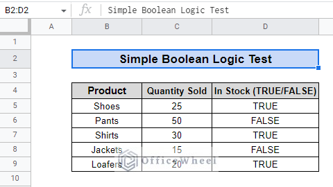
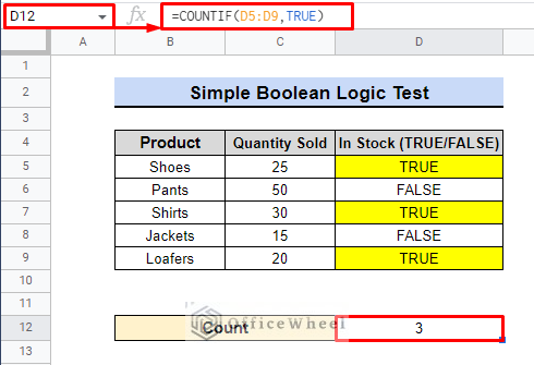
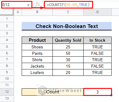
The dataset we have contains information about products and their quantity sold. It also has a column indicating whether the product is currently in stock or not, represented by the values “TRUE” or “FALSE“. To find out how many of the products are in stock, we will use a formula to count the number of times the value “TRUE” appears in the stock column.
Steps:
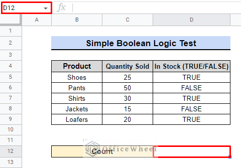
- Firstly, we will select cell D12.
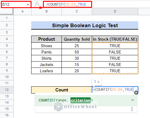
- Secondly, we will use the following formula to count the TRUE Values.
=COUNTIF(D5:D9,TRUE)- Lastly, pressing ENTER will bring forth the result.
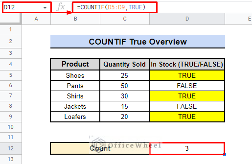
The result of this formula is “3” as we can see in the image provided, indicating that there are three products currently in stock.
Read More: [Fixed!] COUNTIF Function Is Not Working in Google Sheets
2. Values with Checkbox
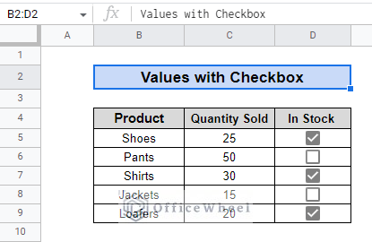
Consider that we have a similar dataset. However, Instead of using TRUE or FALSE values, the dataset now uses checkboxes to identify whether the product is still in stock or not.
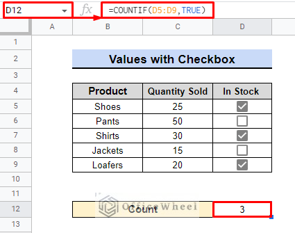
We will use the same formula as before to count the number of products that are marked as in stock by checking for true values in the “In Stock” column.
Steps:
- Initially, we will select cell D12.
- Subsequently, we will use the following formula.
=COUNTIF(D5:D9,TRUE)- Ultimately, press ENTER to see the result.
Initially, by examining the image, we can see that the result is 3. This indicates that there are three products currently in stock.
Read More: Use COUNTIF Function to Count Checkbox in Google Sheets
Similar Readings
- How to Execute Case Sensitive COUNTIF in Google Sheets
- COUNTIF with Greater than and Less than Criteria in Google Sheets
- How to Use VLOOKUP with COUNTIF Function in Google Sheets
3. Check Non-Boolean Text
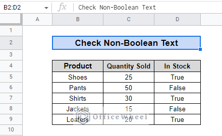
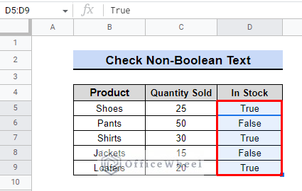
While working on google sheets, we will come across some situations where there will be non-boolean texts such as True or False. The COUNTIF function can only count cells that have a boolean value, so if the cells in the range contain non-boolean values, the function will not be able to count them.
The True and False values that you see in the image above are text values, not Boolean.
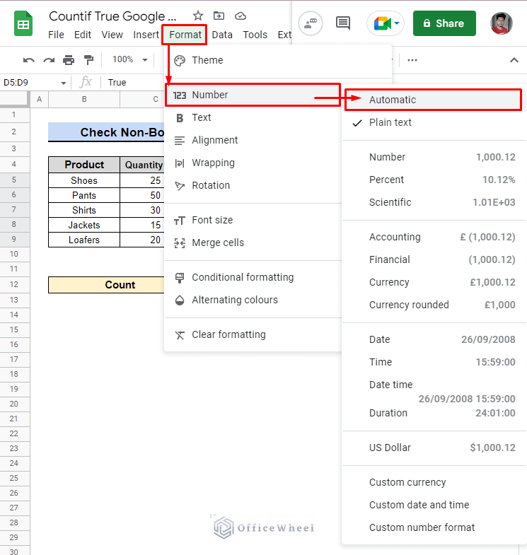
To make the COUNTIF function count the values in the “In Stock” column, we must format the column first. Check the following steps to understand.
Steps:
- First, we need to select the data range of the “In Stock” column.
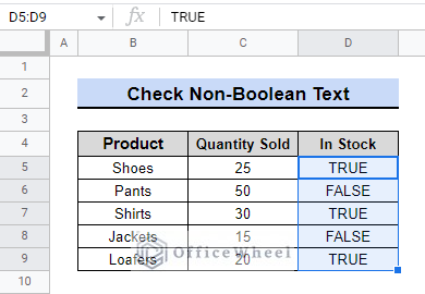
- Afterward, we will change the data format to Automatic. Therefore, it will convert the non-boolean True or False text into Boolean TRUE or FALSE.
- The resulting dataset looks like this:
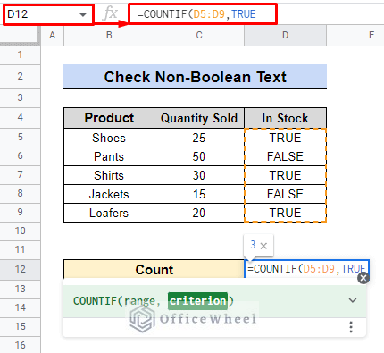
- Now, we will select cell D12 to apply the following formula.
=COUNTIF(D5:D9,TRUE)- In the end, press ENTER to see the result.
We can adjust the dataset to make the COUNTIF function count the values in the “In Stock” column by changing the data format from Plain text to Automatic. This will convert non-boolean text into boolean text values and provide an accurate outcome.
Read More: Google Sheets Count Cells from Another Workbook with COUNTIF Function
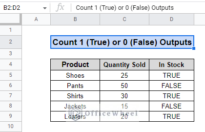
4. Count 1 (True) or 0 (False) Outputs
We can convert boolean text or checkboxes into numerical values, such as 1 and 0, in Google Sheets using the ARRAYFORMULA function. This allows us to easily use these values in calculations and functions like COUNTIF.
Steps:
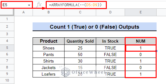
- We will begin by creating a new column and labeling it as NUM.
- Afterward, we will select cell E5 and use the following formula.
=ARRAYFORMULA(--(D5:D9))- This formula uses the ARRAYFORMULA function to convert any TRUE or FALSE values in the range D5:D9 to 1 or 0 respectively, by using a double negation (—) operator.
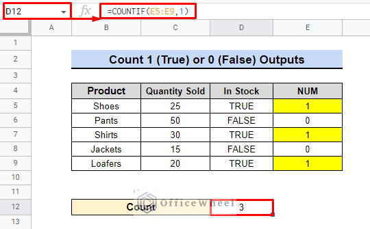
- Next, in order to count the number of TRUE values, we’ll select cell D12 and input the following formula.
=COUNTIF(F5:F9,1)- Press ENTER to apply.
The formula yields the same result as before, which is 3, indicating that there are three products in stock.
Read More: How to Use COUNTIF Function with OR Logic in Google Sheets
Conclusion
The COUNTIF function in Google Sheets with the TRUE or FALSE Boolean criteria allows for powerful data analysis in a business setting. With the ability to quickly and easily count the number of times, certain criteria are met. The function’s flexibility and simplicity make it a valuable tool for any business looking to gain insights from its data. For more insight check our website OfficeWheel.

