How to Use Weighted Average Formula in Google Sheets

We generally use the weighted average in those places where calculating the normal average would give a false result. Using the weighted average formula in Google Sheets is pretty straightforward. There is a function built in at Google Sheets that give the weighted average directly. The function is called the AVERAGE.WEIGHTED function. We can also use the combination of the SUMPRODUCT and SUM functions to calculate the weighted average in Google Sheets. In this article, I’ll show you 5 suitable examples to use the weighted average formula in Google Sheets with clear steps and images.

A Sample of Practice Spreadsheet

You can download Google Sheets from here and practice very quickly.

5 Suitable Examples to Use Weighted Average Formula in Google Sheets

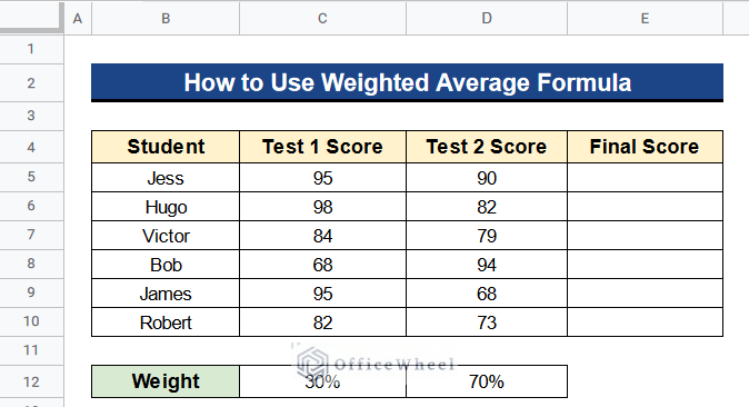
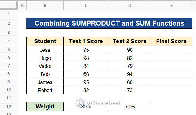
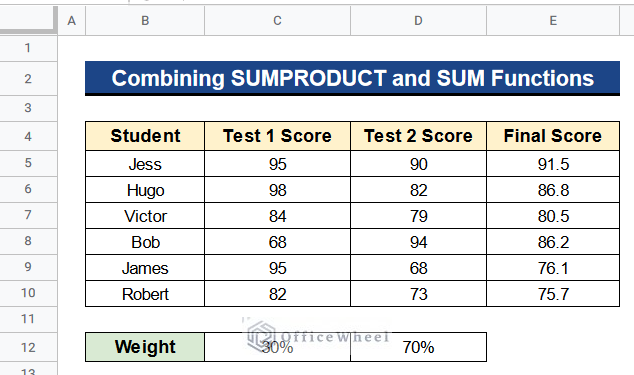
Let’s get introduced to our dataset first. Here we have some students in Column B and their test scores in Column C and Column D. Separate weights have been given on each test score in Column C and Column D as we can see in the picture. Now we have to calculate the final score of every student. The final score would be the weighted average of their 2 separate tests. So we’ll see 5 useful examples to use the weighted average formula in Google Sheets.

Example 1. Using AVERAGE.WEIGHTED Function with Weight in Percentage

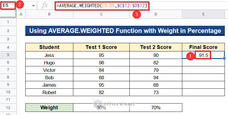
In our dataset, the weights are given as percentages. So now we’ll see how to calculate the weighted average of every student’s score using the AVERAGE.WEIGHTED function. This function does 2 things together. First, it multiplies each test score by its weight. Then it simply divides them with the summation of the weights. Finally, we’ll get our desired output very quickly.

Steps:

• Firstly, type the following formula in Cell E5–

• Secondly, hit Enter to get the weighted average.

• Thirdly, apply the Fill Handle tool to use the formula in the rest of the cells of the column.

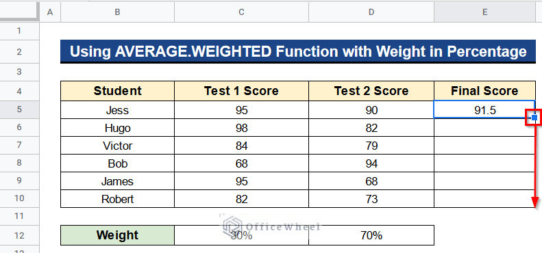
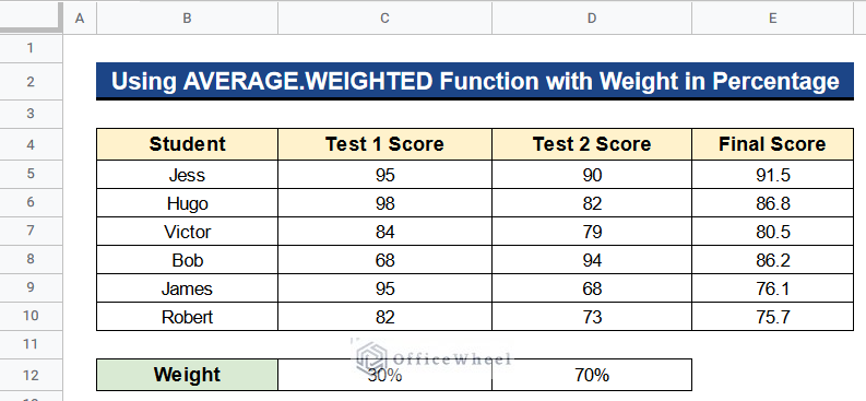
• Finally, you’ll get the final scores of all the students, which are the weightage averages of 2 test scores.

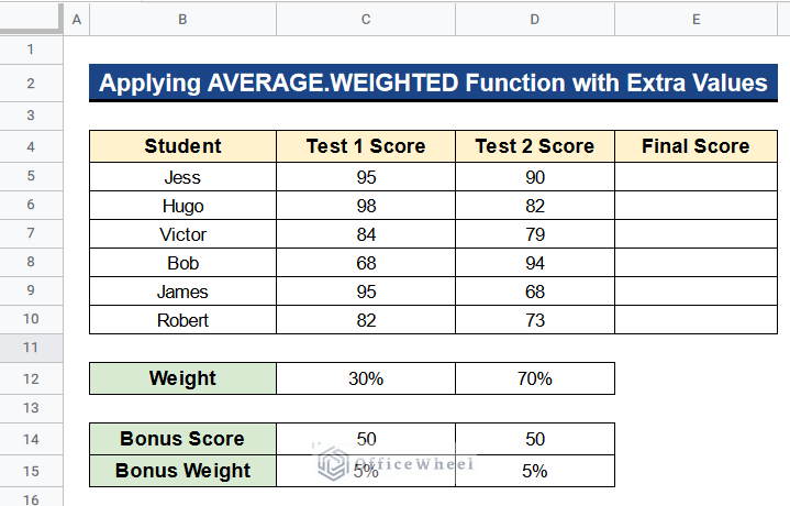
Example 2. Applying AVERAGE.WEIGHTED Function with Extra Values

Additionally, we can extend the AVERAGE.WEIGHTED function if we have extra values like in our case. At this time we have bonus score and bonus weight in Column C and Column D. We want to add them to our calculation. So putting these values simply into our formula will do the job. Let’s see how to do that.

Steps:

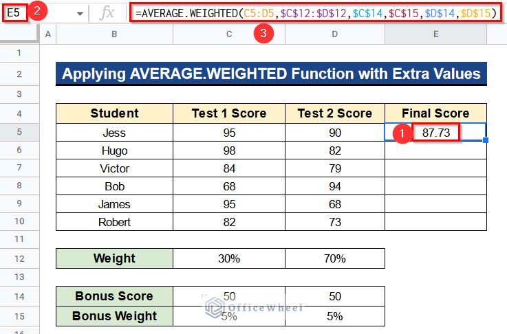
• At first, write the next formula in Cell E5–

• Then, press Enter to get the final score.

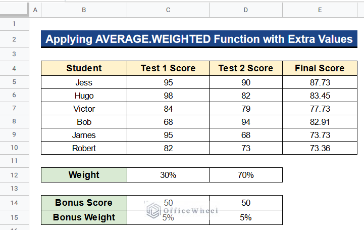
• At last, use the Fill Handle tool to apply the formula in all cells. In the end, you’ll get your desired result.

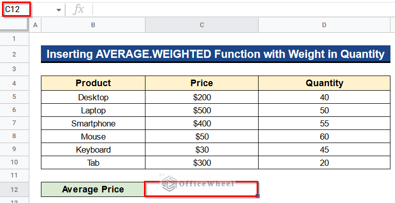
Example 3. Inserting AVERAGE.WEIGHTED Function with Weight in Quantity

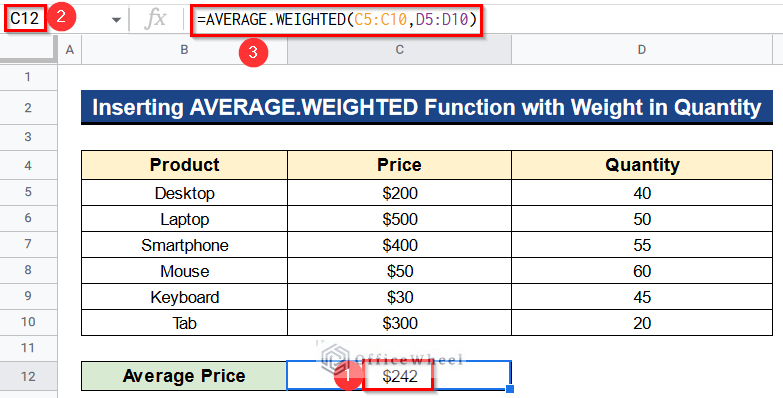
Look at some different problems this time. We have some products in Column B, their prices in Column C, and their quantity in Column D. Now, we’ll use those quantities as weight and we want the total weighted average price of those products. Let’s solve this problem using AVERAGE.WEIGHTED function.

Steps:

• First, insert the below formula into Cell C12–

• Ultimately, hit the Enter Button to obtain the weighted average price of the products.

Example 4. Combining SUMPRODUCT and SUM Functions

Moreover, we can use the combination of SUMPRODUCT and SUM functions to calculate the weighted average in Google Sheets. The SUMPRODUCT function will first multiply each test score by its weight and add them together. Then we’ll divide these products with the summation of the weights using the SUM function. This process is a bit longer because we have to use 2 functions here.

Steps:

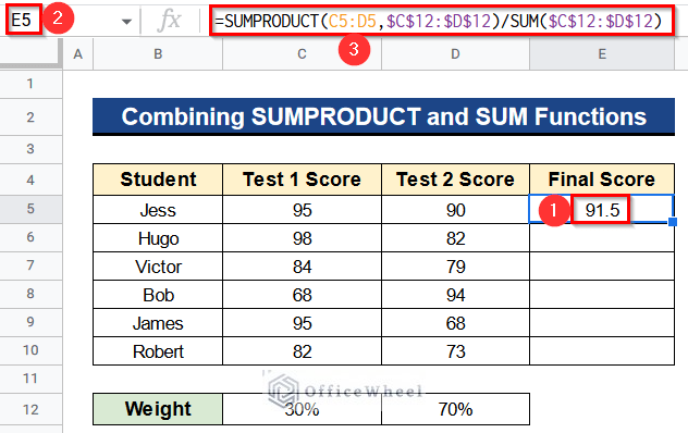
• Before all, type the next formula in Cell E5–

• Consequently, press the Enter Button to get the weighted average of the scores.

• Then, apply the Fill Handle tool to get the output in the whole column.

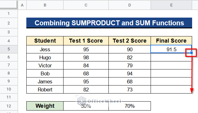
• Finally, we’ll get our final scores like this picture.

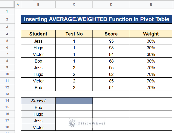
Example 5. Inserting AVERAGE.WEIGHTED Function in Pivot Table

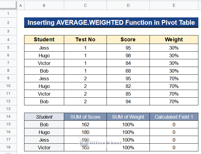
We use the Pivot Table in Google Sheets to calculate and analyze data quickly. We can insert the AVERAGE.WEIGHTED function in Pivot Table. Here we have a dataset having students’ names in Column B, their test no in Column C, their scores in Column D, and their weight in Column E. And we also have a Pivot Table having only the unique students’ names in Column B. Now we’ll see how to calculate the weighted average using Pivot Table in Google Sheets.

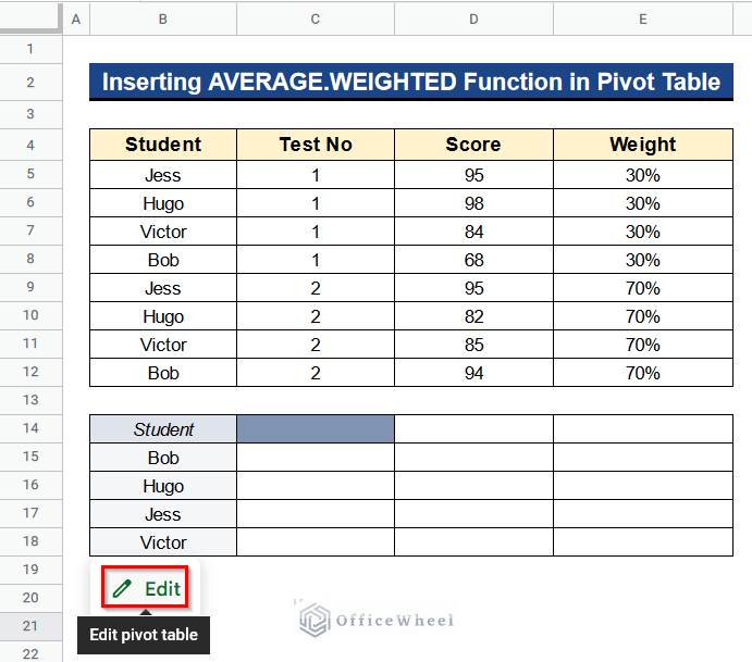
Steps:

• Earlier on, click on the Edit Button situated under the Pivot Table to go to Pivot Table Editor as shown in the picture.

• Moreover, in the Pivot Table Editor Box click on Add under the Values menu and add Score, Weight, and Calculated Field.

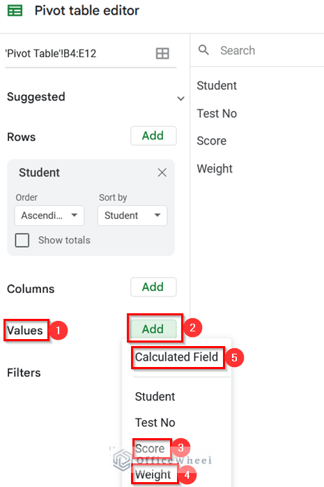
• Consequently, you’ll get a Pivot Table like this.
• Now, we’ll calculate the weighted average in the Calculated Field 1 Column.

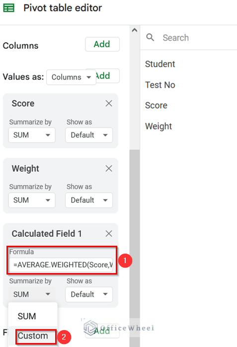
• Again go to Pivot Table Editor Box and type the following formula in the formula box under the Calculated Field 1 menu-

• Next select Custom under Summarize By menu.

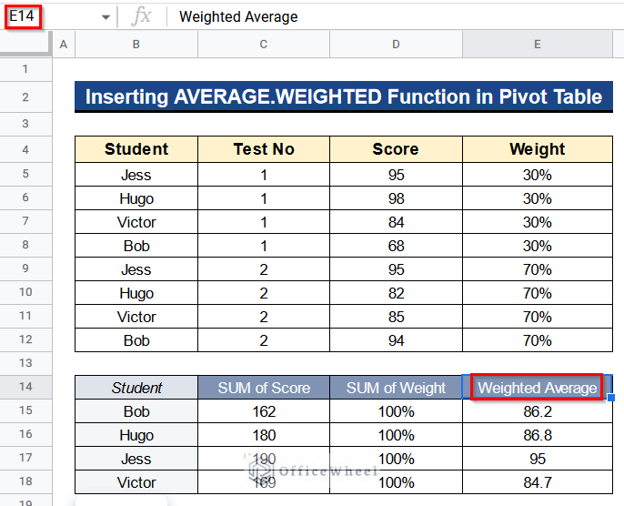
• In the end, we’ll get the weighted average in the Pivot Table.
• Don’t forget to rename Cell E14 as Weighted Average.

Read More: Calculate Weighted Average Using Pivot Table in Google Sheets

Weighted Average Calculator

Last but not least we can create a weighted average calculator in Google Sheets. In that calculator when we put any values and their weights, it’ll give results directly. Below you’ll find the steps for creating the weighted average calculator.

Steps:

• Initially, type the following formula in Cell C12–

• Then, hit the Enter Button to get something like the picture.

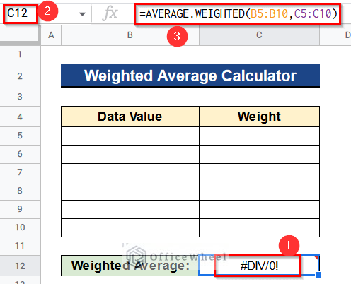
• When we put any values in this calculator, it’ll produce results automatically. As we haven’t put any values it is showing an error message. Nothing to worry about for this.

Conclusion

That’s all for now. Thank you for reading this article. In this article, I have discussed how to use the weighted average formula in Google Sheets with 5 useful examples. I have also discussed creating a weighted average calculator. Please comment in the comment section if you have any queries about this article. You will also find different articles related to google sheets on our officewheel.com. Visit the site and explore more.

Related Articles

• How to Calculate Conditional Weighted Average in Google Sheets
• Calculate Weighted Average Using IF Function in Google Sheets
• How to Calculate Weighted Average in Google Sheets