The Pivot Table is a renowned feature in Google Sheets. We can do multiple calculations through the Pivot Table. In this article, we’ll see 2 easy methods to calculate weighted average using Pivot Table in Google Sheets. For this purpose, we’ll use the AVERAGE.WEIGHTED function and combination of SUMPRODUCT and SUM functions.
A Sample of Practice Spreadsheet
You can download Google Sheets from here and practice very quickly.
What Is Weighted Average?
Foremost, we have to know what is a weighted average. We know about the simple average but the weighted average is quite different. Sometimes during calculation, we have to put weights on values. The weighted average takes into account the weight given to a certain value and gives the average of the values. It simply multiplies every value by its weight and divides them by total weight.
2 Easy Methods to Calculate Weighted Average Using Pivot Table in Google Sheets
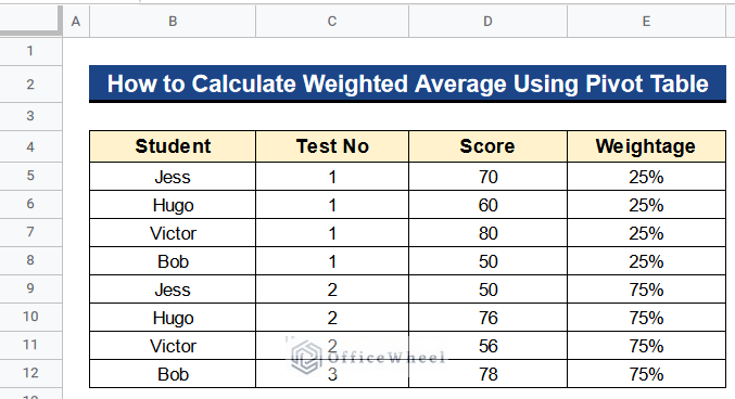
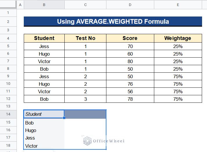
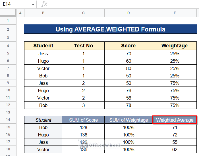
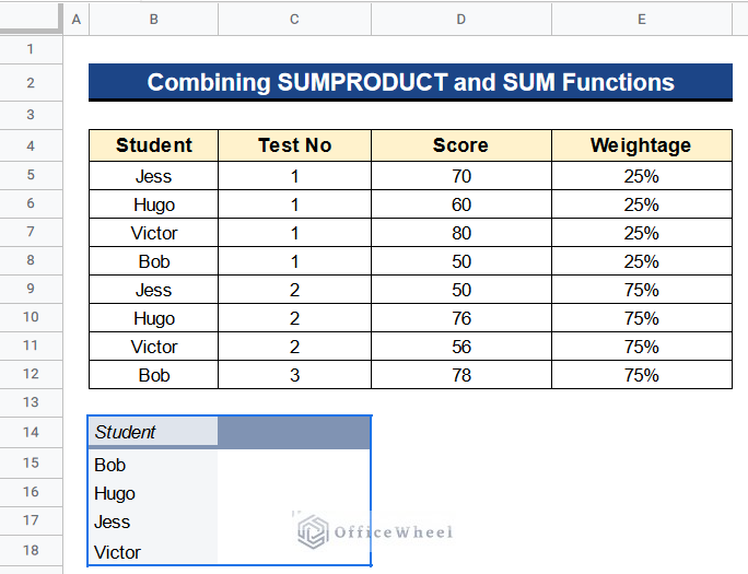
Let’s get introduced to our dataset first. Here we have some students’ names in Column A, test numbers in Column B, test scores in Column C, and weightage given on each test score in Column D. Now we want to calculate the weighted average using the Pivot Table in Google Sheets. We’ll use 2 simple methods to calculate the weighted average.
1. Using AVERAGE.WEIGHTED Formula
There is a simple formula in Google Sheets to calculate the weighted average. The function is called the AVERAGE.WEIGHTED function. This function directly gives the weighted average based on the given criteria. We’ll use this formula in the Pivot Table to calculate the weighted average. In our case, this formula will directly take values from the Pivot Table which are Score and Weightage, and calculate them to give the result.
Steps:
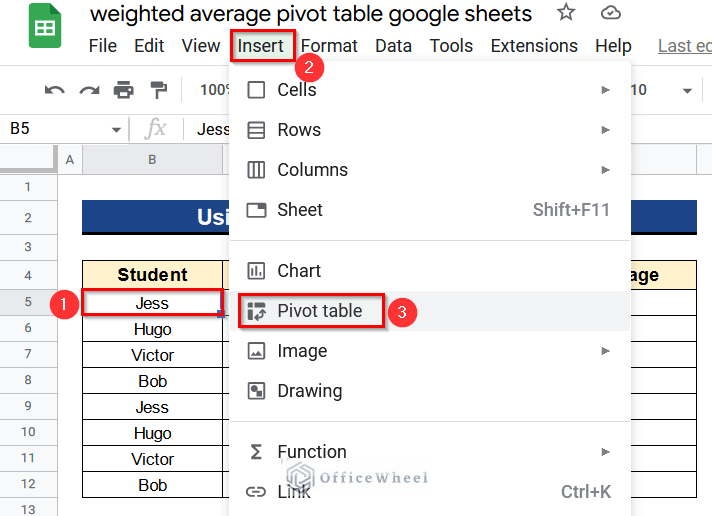
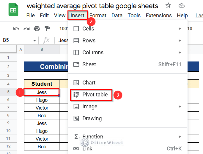
- Firstly, select Cell B5 in the dataset and go to Insert > Pivot Table.
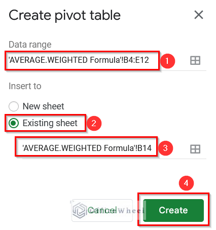
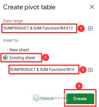
- Secondly, give data range from Cell B4 to E12.
- Thirdly select the Existing Sheet Button and give the position where the Pivot Table would start. In our case, it is Cell B14.
- Then click the Create Button.
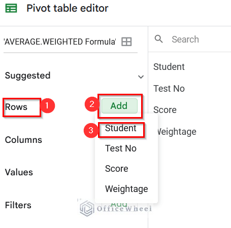
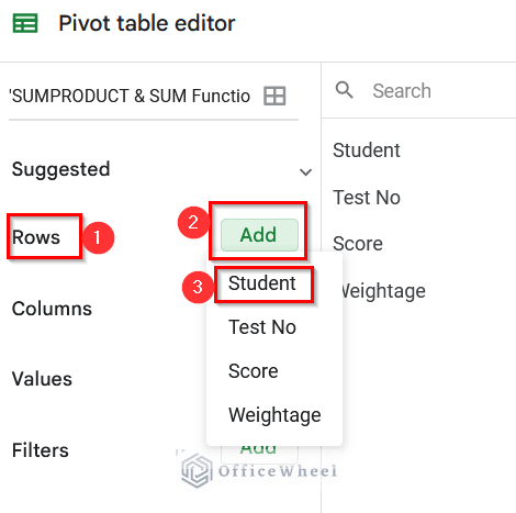
- After that, under the Rows menu click Add Button in the Pivot Table Editor box and select Student from there.
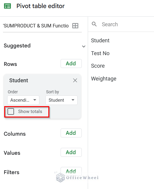
- Moreover, remember to untick the Button beside Show Totals.
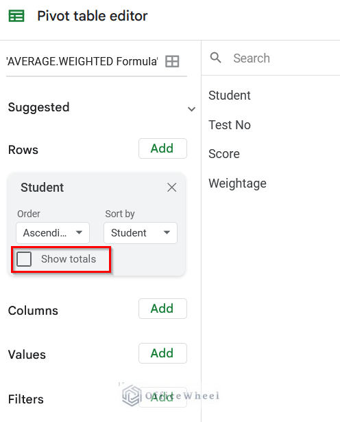
- Finally, the Pivot Table will be created having the student’s name in rows.
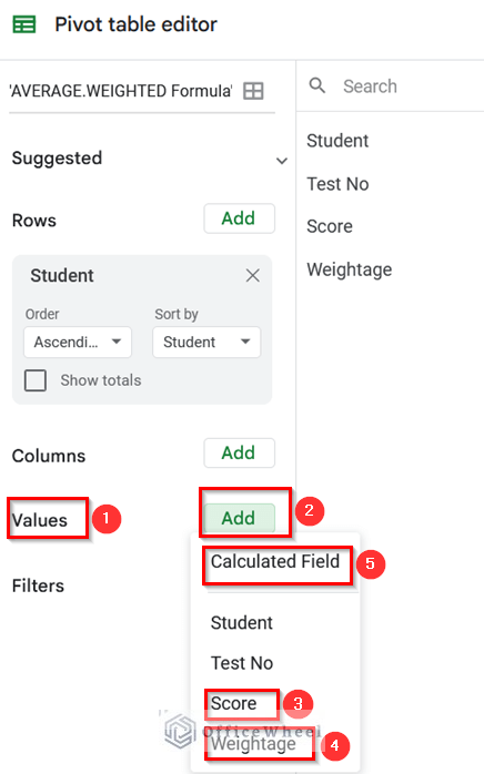
- Again go to the Pivot Table Editor box.
- Then select Add Button under the Values menu and select Score, Weightage, and Calculated Field serially from there.
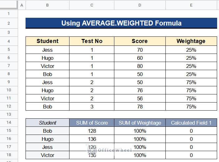
- At last, you’ll get the output like the one below.
- Now we’ll calculate the weighted average of the scores.
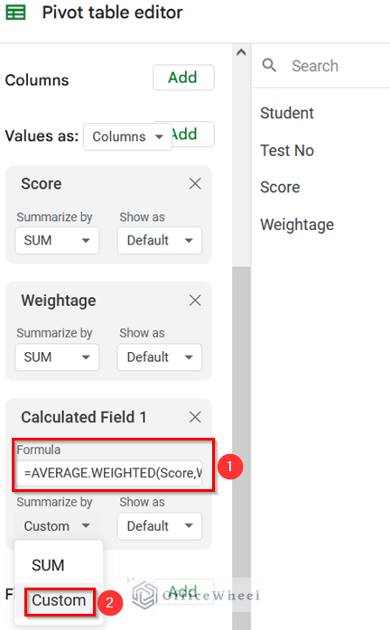
- For that reason, again go to the Pivot Table Editor menu. Then, under the Calculated Field 1 menu type the following formula into the formula bar-
=AVERAGE.WEIGHTED(Score,Weightage)- In addition select Custom under Summarize By menu.
- In the end, you’ll get the weighted average of the scores.
- At last, we renamed Cell E14 as Weighted Average.
Read More: How to Use Weighted Average Formula in Google Sheets
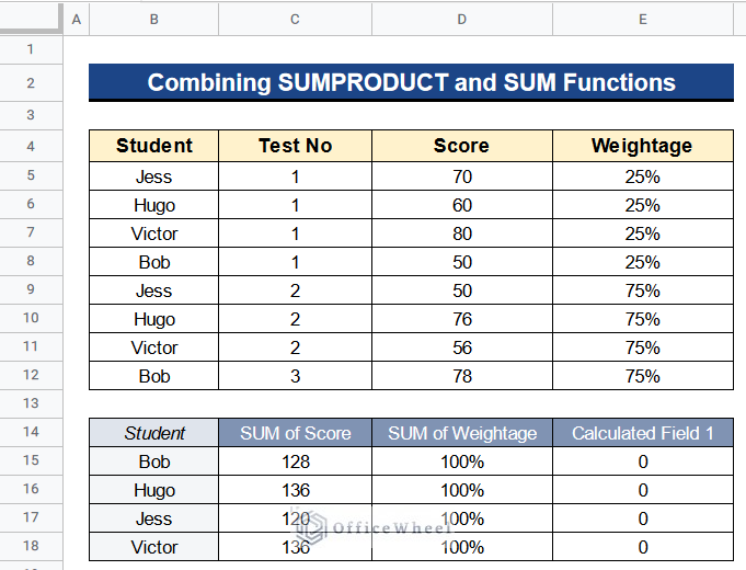
2. Combining SUMPRODUCT and SUM Functions
Unlike the previous method, we can also combine 2 functions, SUMPRODUCT, and SUM functions to calculate the weighted average using the Pivot Table in Google Sheets. These 2 functions together do the same task as the former method.
Steps:
- First of all, select any cell from the dataset. In our case, it is Cell B5.
- Next, go to Insert > Pivot table.
- Afterward, we’ll give our data range which is from Cell B4 to E12.
- Hence select the Existing Sheet Button and give the position as Cell B14.
- After that select the Create Button.
- Moreover, go to the Pivot Table Editor box.
- Then, click Add Button under the Rows menu and select Student.
- Don’t forget to uncheck the box beside Show Totals.
- In the end, you’ll get a Pivot Table that has the student’s name in Column B.
- Next, go to the box titled Pivot Table Editor.
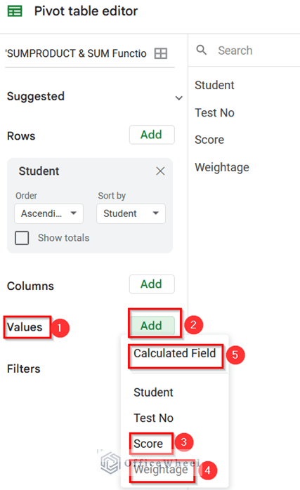
- After that click on the Add Button near the Values menu.
- Then, select Score, Weightage, and Calculated Field serially as shown in the picture.
- Consequently, we’ll get the full Pivot Table.
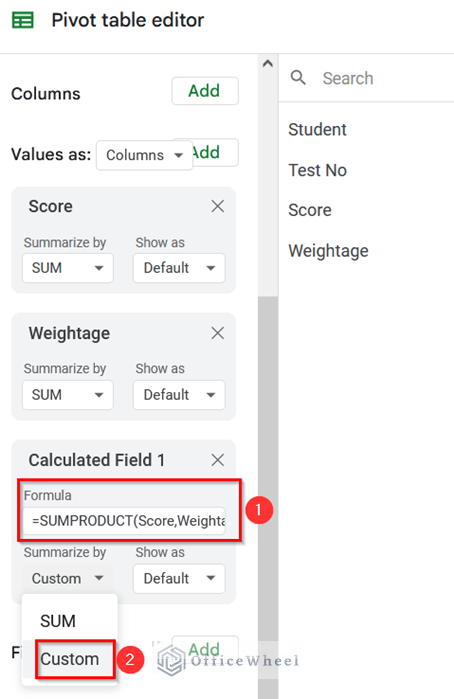
- Next, go to the Pivot Table Editor menu.
- Hence, type the following formula into the Formula Box–
=SUMPRODUCT(Score,Weightage)/SUM(Weightage)- Further, click on Custom under the Summarize By menu.
Formula Breakdown
- SUMPRODUCT(Score, Weightage)
At first, this function multiplies Score by Weightage and after that, it adds the products of Score and Weightage.
- SUM(Weightage)
Then we use this function to divide the sum-product values of Score and Weightage by the sum of Weightage. Which eventually gives us the weighted average.
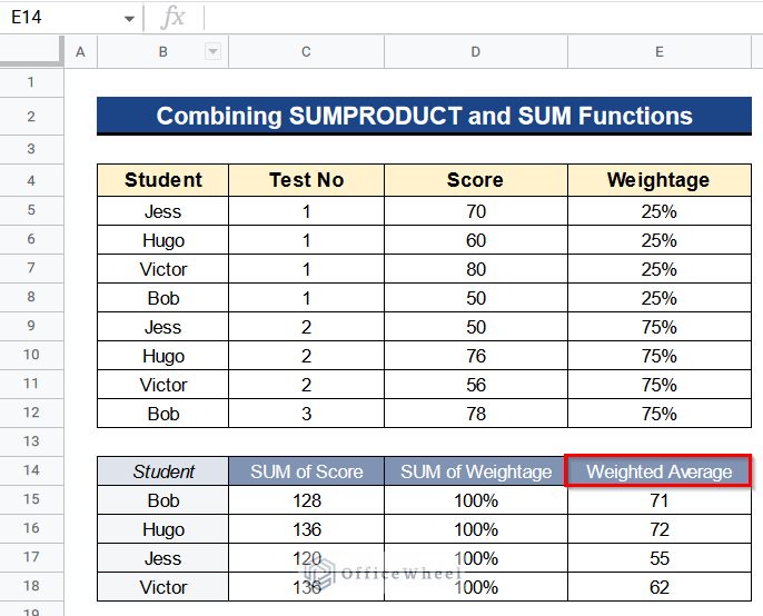
- Finally, we’ll get our desired result.
- Last, rename Cell E14 as Weighted Average.
Advantage of Calculating Weighted Average in Google Sheets
In our dataset, there are scores for 2 different tests. Each test has separate weightage, 25%, and 75%. Now, we want to know the average score of any student. So, if we take the normal average, it would be wrong. In this case, the weighted average serves the purpose easily. This is the advantage of calculating the weighted average.
Conclusion
That’s all for now. Thank you for reading this article. In this article, I have tried to discuss 2 quick methods to calculate the weighted average using Pivot Table in Google Sheets. Please comment in the comment section if you have any queries about this article. You will also find different articles related to google sheets on our officewheel.com. Visit the site and explore more.