Create Drop Down List in Google Sheets from Another Sheet

Google Sheets drop-down list is very useful when you want to enter data from some predefined options. The drop-down list is one of the efficient ways of data entry and can make the process consistent and error-free. In this article, we are going to know how to create Google Sheets drop-down list from another sheet.

Table of Contents

A Sample of Practice Spreadsheet

You can download the spreadsheet to practice.

Create a Dropdown List from Another Sheet

Step-by-Step Procedure to Create Drop-Down List in Google Sheets from Another Sheet

For creating a drop-down list in google sheets by using data from another sheet, first of all, we select a source dataset from where the drop-down list will be developed, then import the data in a new sheet, and finally through data validation create a drop-down list for our target dataset using the source dataset.

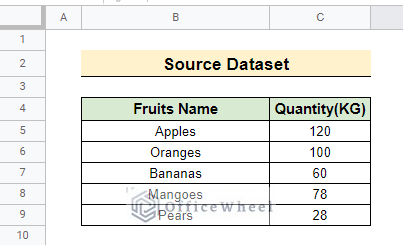
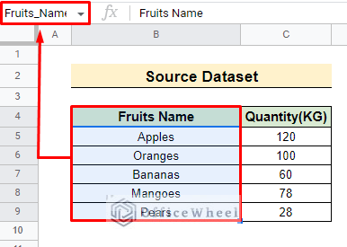
The source dataset represents two columns namely Fruits Name and Quantity.

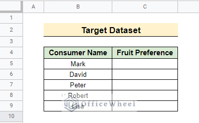
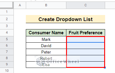
And the target dataset which displays on another spreadsheet presents two columns named Consumer Name and Fruit Preference.

Step 1: Create a Named Range in the Source Dataset

Before creating a drop-down list, we will be naming the data range that we will import from spreadsheet 1. The source dataset is a dataset from where we will use data for the drop-down list.

Here, the dataset contains two specific columns. The first column represents the Fruit Name and the second one presents its quantity.

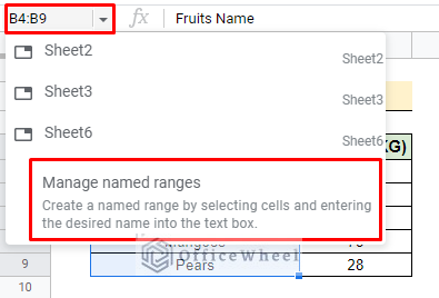
Create a named range for the Fruits Name column range “Fruits_Name”.to do so, first select the whole column or cell range that you want to name. Then go to the Manage named ranges.

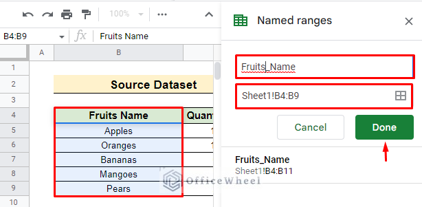
Then change the name. Here, we name the range “Fruits_Name”. Then press Done.

When you select the range, you can see the name range above there.

Step 2: Import Data from Another Sheet

To import data in another sheet some steps should be followed:

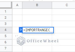
Open the target worksheet (spreadsheet 2) and create a new worksheet in it. Insert “=IMPORTRANGE (“ formula into a selected cell.

The formula syntax is

=IMPORTRANGE("<URL>","Sheet1!Fruits_Name")

Here, URL is the unique ID that Google Docs assigns for each spreadsheet.

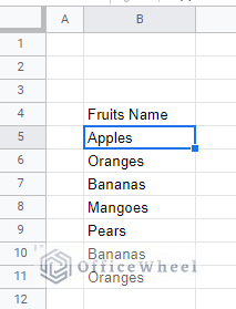
=IMPORTRANGE("https://docs.google.com/spreadsheets/d/1CoSFP07_IdCrHnTIkMEw01fPrI87c9kqy6XMLQccdVI/edit#gid=0","Sheet1!Fruits_Name")

Press ENTER and you will find the Fruit_Name column import from the source dataset into the new Google Sheets.

Note: This step is not necessary if the data is only in a separate worksheet in the same spreadsheet since you can directly apply data validation (Step 3) if the data is in the same spreadsheet.

Step 3: Create Drop-Down List for the Target Dataset

We already have a target dataset containing two columns, namely Consumer Name and Fruit Preference. In the Fruit Preference column, we will add the drop-down list beside each consumer name so that the user can select it independently.

To create a drop-down list,

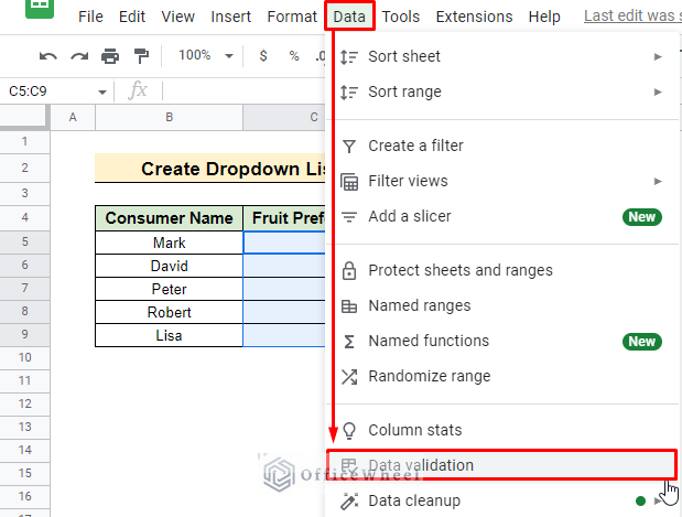
First, select the cells or column you want to add to a drop-down list.

Then go to Data and select Data validation.

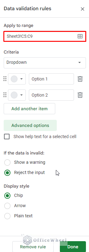
The apply range is default selected as we select the cells before going to the data validation tab.

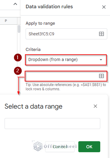
Enter Criteria: Dropdown (from a range) and then go to select a data range.

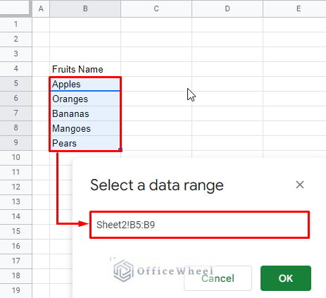
Select the data to range from imported data in Sheet2.

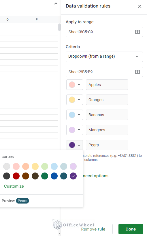
After selecting data, you can find all the values for the drop-down list in the data validation bar. A color customization bar will automatically add to your drop-down values. You can customize the color for each value to mark them separately.

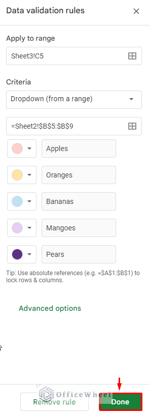
Press Done to run the method.

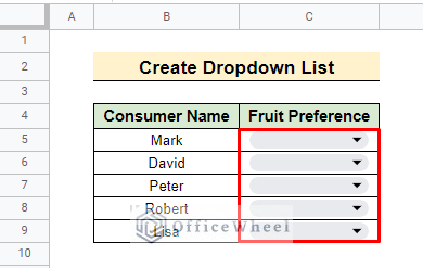
You can find the drop-down in the desired column that we have selected.

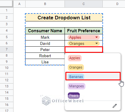
Now you can select any options for your desired cells.

Things to Remember

For Import data, the URL must be put properly.
For data validation, you have to select the ranges carefully.

Conclusion

Now you can easily create a Google Sheets dropdown list from another sheet and can make your dataset more effective for different purposes. To explore more techniques, you can visit our OfficeWheel website. Feel free to comment if you have any queries.