How to Average in Google Sheets If Value Is Not 0 (2 Simple Ways)

In mathematical calculations, the average plays a significant role. When calculating the average, it could bias the data if we count zero. As a result, understanding how to use Google Sheets AVERAGE is similarly crucial for accuracy and fairness, if not even zero (0). This post will show you how to average data from Google Sheets when it contains zeros.

Table of Contents

A Sample of Practice Spreadsheet

You can copy the spreadsheet that we’ve used to prepare this article.

AVERAGE If Not Zero

Why We Cannot Ignore Zero (0) in AVERAGE Function in Google Sheets

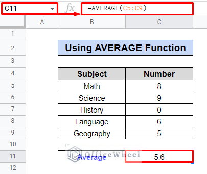
The Google Sheets AVERAGE function typically counts all values, including zero, with the exception of empty cells and text values. Check the following example.

Fundamentally, the syntax of the AVERAGE function only accepts values or a range. Even if we wanted to exclude zero, we couldn’t do so using the AVERAGE function because it doesn’t need any conditions or criteria.

As a result, it included zero and generated a score of 5.6 on average.

However, the good thing is, in Google Sheets, there are two simple ways to determine the average by overcoming this issue.

2 Simple Ways to Average in Google Sheets If Value Is Not (0)

1. Application of AVERAGEIF Function

AVERAGEIF is the appropriate function to utilize if we wish to exclude zero from the average calculation. This post will demonstrate the procedures using a clear and simple example.

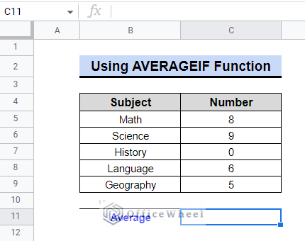
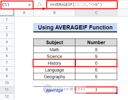
Consider that we have data on the most recent class test of a student. We intend to find the average score for the five subjects.

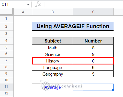
It should be noted that we may overlook any subject if the result is zero in order to measure the overall performance.

Steps:

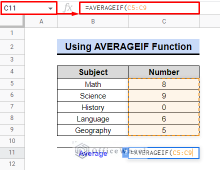
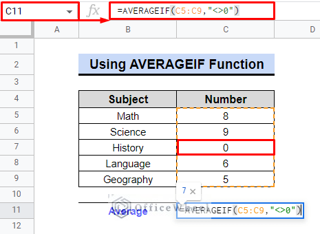
Select cell C11 first.
We’ll employ the AVERAGEIF function. In this instance, the criterion range is C5:C9, and we need to place it first.

The condition now is to exclude 0. Therefore, we will use “<>0” to indicate that we do not want to use zero values while averaging the values within the specified cell range.
The final equation is thus:

=AVERAGEIF(C5:C9,"<>0")

We can get your answer by pressing ENTER.

If we mathematically check the equation, the total sum is 28. Now, if we disregard the zero, we must also ignore the subject count.

As a result, We will receive a final score of 7, which is the average of the remaining four.

If we add the zero, it will be 5.8, nevertheless.

As proof, we now realize that AVERAGEIF and “<>0” is the appropriate expression to utilize if we want to use Google Sheets average in cases of if not zero.

2. Use of AVERAGE & QUERY Functions

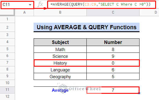
To ignore 0 numbers, we may alternatively combine the QUERY function with the AVERAGE function. We will use the QUERY function to add criteria within the AVERAGE function since the AVERAGE function is unable to contain any conditions or criteria. The QUERY function will work as a filter here so that we can get values that are greater than zero (0). We’ll show you how to do it using the same database.

Steps:

First, select cell C11.
Secondly, use the following formula:

=AVERAGE(QUERY(C3:C9,"SELECT C Where C >0"))

Press ENTER, finally, to get the result.

Formula Explanation:

QUERY function
- The data range for the QUERY function is C3:C9.
- “SELECT C Where C >0” returns values larger than 0 in column C.
AVERAGE function
- Averages the values returned by the QUERY function.

NOTE: The value for the query must either be a reference to a cell containing the required content or be contained in quotation marks.

Conclusion

With this knowledge, you may quickly calculate your average in Google Sheets without distorting your data. While conducting significant analysis, it’s crucial to have a proper comprehension of mathematical equations. One of the cases is Google Sheets AVERAGE if the value is not zero (0).

Visit OfficeWheel to read more articles on Google Sheets average.