You can regularly find yourself searching through data in Google Sheets to locate a specific text. On smaller spreadsheets, this can be accomplished manually with ease. However, large spreadsheets make this almost impossible. Fortunately, Google Sheets has a variety of built-in tools that make it simple to do text searches within the worksheets. In this article, we will show you 4 simple ways to search for text in range in Google Sheets.
4 Simple Ways to Search for Text in Range in Google Sheets
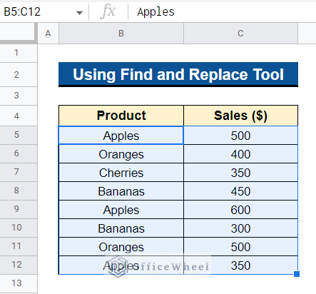
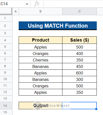
The dataset below will be used to demonstrate the example of searching for text in range in Google Sheets. The dataset contains the product name and sales of the product of a shop. We want to search for the product name here.
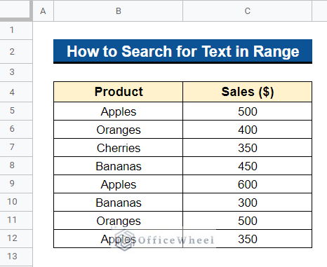
1. Using Find and Replace Tool
The Find and Replace tool in Google Sheets search the spreadsheet for the specified term. Case matching is one of the biggest benefits it offers over utilizing formulae to accomplish the same goal.
Steps:
- First, select the data range from where you want to search your specific text. We selected Cell B5:C12.
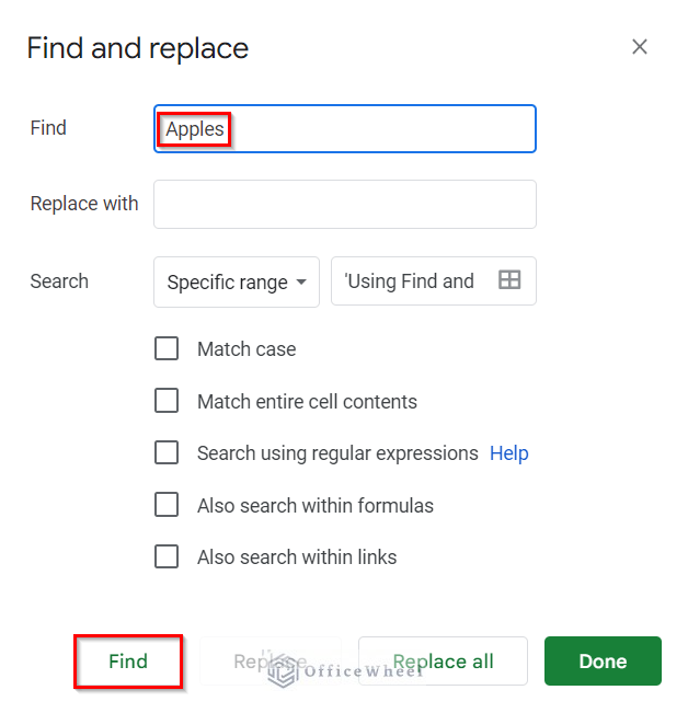
- Now, press the Ctrl+H button to open up the Find and replace dialog box. Then, type the specific text you want to search in the Find box.
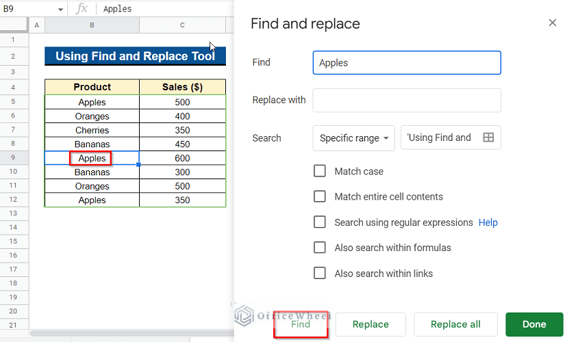
- Now, click on Find It will go to the precise text in the data range you searched for.
- To repeatedly discover your particular text, click the Find button again and again. After searching the text, you can click the Done button to remove the dialog box.
Read More: How to Search and Replace in Google Sheets (2 Easy Ways)
2. Applying Conditional Formatting
We can use Google Sheets’ Conditional Formatting feature to search for text in range. You can search for specific text and highlight it by color using this feature.
Steps:
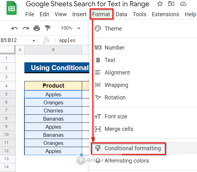
- First, select the data range. Go to the Format tab from the top menu bar and select Conditional formatting.
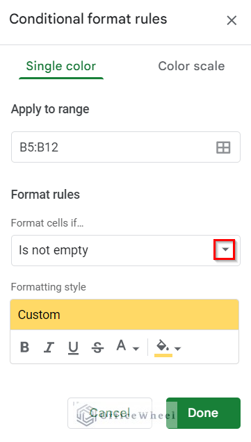
- The Conditional format rules dialog box will open up. Click on the drop-down icon in Format cells if… box.
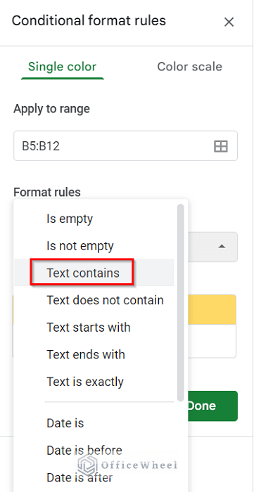
- Now, select Text contains from the Format cells if… box.
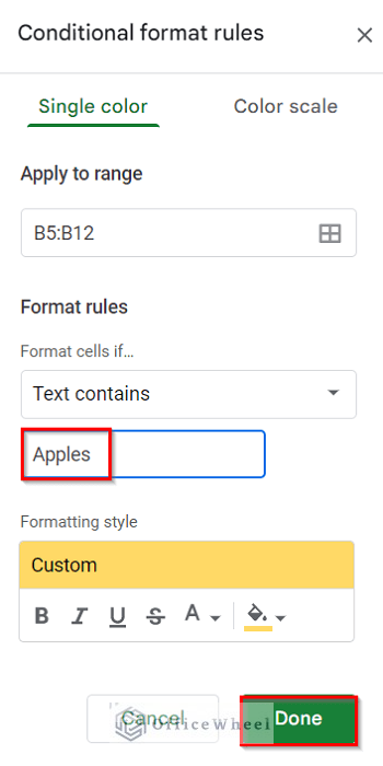
- Now, type the specific text you want to search for on the Values option and press Done.
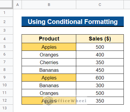
- All of the cells that contain the specified text are now highlighted.
3. Employing MATCH Function
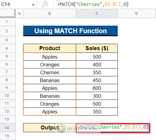
In Google Sheets, the MATCH function is another technique to search for text inside a range. When a user-specified value matches one in a specific cell range, the MATCH function returns the relative location of that value based on the selected range.
Steps:
- First, select a cell where you want the output. We selected Cell D5.
- Now type the formula below and press the Enter button-
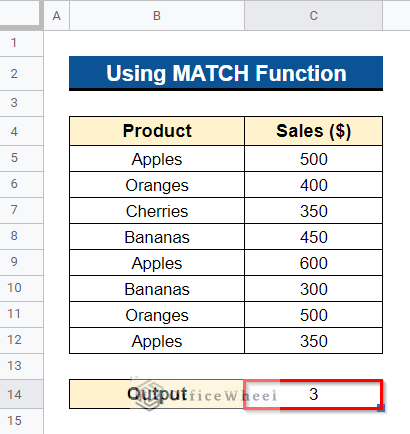
=MATCH("Apples",B5:B12,0)- The specific text we were looking for is present in the 3rd row. It will show you the result of the first occurrence of your specific text.
4. Using LOOKUP Functions
In Google Sheets, we may utilize the LOOKUP functions to search for text inside a range. The required outcome will be displayed by LOOKUP functions once they have compared your data from one range to another.
4.1 LOOKUP Function
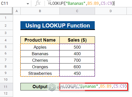
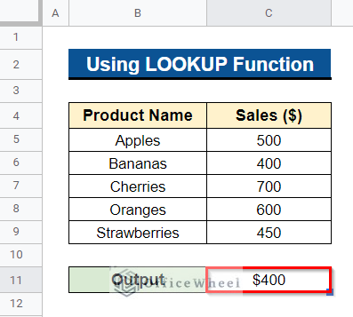
We can use the LOOKUP function to search for text in the range in Google Sheets. The LOOKUP function enables you to compare sorted data from one range to data from another range at the same point.
Steps:
- First, select a cell where you want the output. We selected Cell C11. Type the formula below-
=LOOKUP("Bananas",B5:B9,C5:C9)- Now, press the Enter button and it will show you the sales of the product you searched for.
4.2 VLOOKUP Function
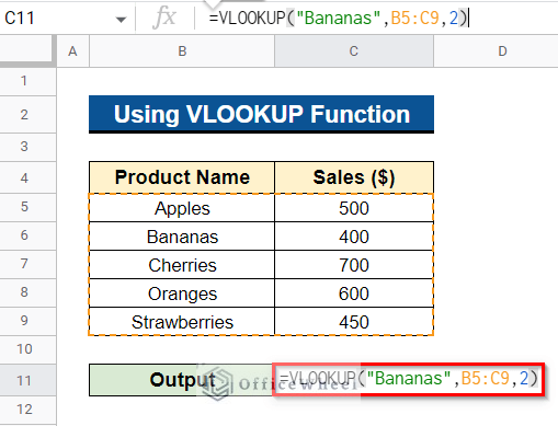
In Google Sheets, we may search for text within a range using the VLOOKUP function. Whether sorted or not, the VLOOKUP function allows you to compare data from one column to data from the same row in another column.
Steps:
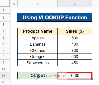
- First, choose the cell that will contain the output. We chose Cell C11. Fill in the formula below-
=VLOOKUP("Bananas",B5:C9,2)- As soon as you press the Enter key, the product’s sales will be shown.
4.3 HLOOKUP Function
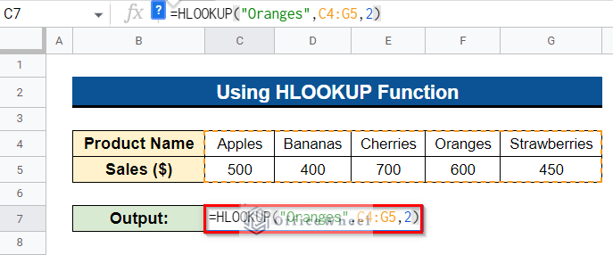
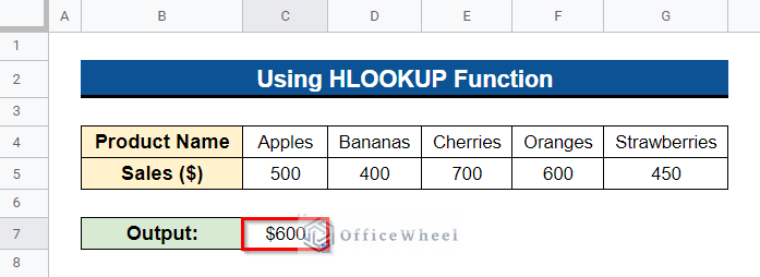
Using the HLOOKUP function in Google Sheets, we may look for text inside a specified range along the row. HLOOKUP can be used to compare data from one row to data from the same column in another row. But the data must be sorted, that’s why we transposed the dataset and sorted it.
Steps:
- First, decide which cell will hold the output. We selected Cell C11. Fill in the following formula-
=HLOOKUP("Oranges",C4:G5,2)- Now, pressing the Enter key will display the product’s sales data.
How to Find Text in a Cell String in Google Sheets
Now we’ll learn how to search text in a string, not in a range. That we can do following two ways
1. Using SEARCH Function
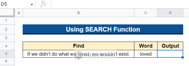
You might occasionally need to know where a certain text is in a string. By using the SEARCH Function, you may accomplish this.
Steps:
- First, select a cell where you want the output to show. We selected Cell D5.
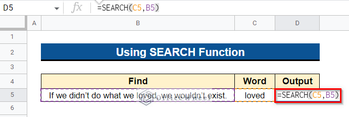
- Now, type the formula below and press the Enter button-
=SEARCH(C5,B5)- Finally, it will show you the position of the specific text within the cell string.
2. Applying FIND Function
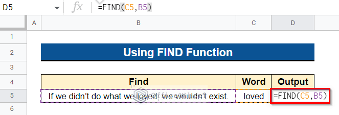
The SEARCH function and the FIND function are nearly identical. We can also use the FIND function to locate the position of a specific text within the cell string in Google Sheets.
Steps:
- First, choose a cell to display the output. We chose Cell D5. Then press the Enter key after typing the formula below.
=FIND(C5,B5)- Finally, it will display where in the cell string the particular text is located.
Conclusion
In this article, we have demonstrated 4 simple ways to search for text in the range in Google Sheets. We have also demonstrated how to locate a specific text within a cell string in Google Sheets. Please feel free to leave any suggestions or ask any questions in the comment section below. Visit Officewheel.com to explore more.

