In today’s article, we will be looking at how to freeze columns in Google Sheets.
Know that the processes are basic and can be used by users of any level of expertise.
But first…
Why should you Freeze Columns?
Freezing columns is crucial when you are handling a wide range of data in your worksheet. As you scroll through these data, the initial important rows or columns will become hidden making you go back to the starting point again to evaluate.
Things can get messy if this continues. And thus, for convenience, we freeze some rows and columns on our worksheet.
Some of the more common scenarios are:
- Compare and contrast data in specific calls to the row or column headers.
- To identify key rows and columns.
- To determine the position of your data throughout the worksheet.
Points to Note
- You cannot freeze rows or columns from the middle of the worksheet.
- You cannot freeze columns and rows simultaneously (at once). Columns must be frozen first then rows, or vice versa.
3 Ways to Freeze Columns in Google Sheets
1. Freeze Columns Using Mouse in Google Sheets (Drag Column Pane)
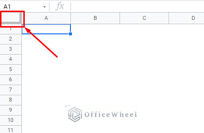
The Row-Column pane is perhaps the most overlooked form for freezing columns or rows in Google Sheets. This is a surprise because it is the simplest way to do so.
You can find it in the top-left former of the worksheet:
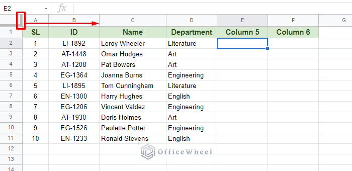
Now, in the following worksheet, we will be using the Column pane (the vertical line) to freeze the SL and ID columns. We do this by clicking and dragging the pane to the right.
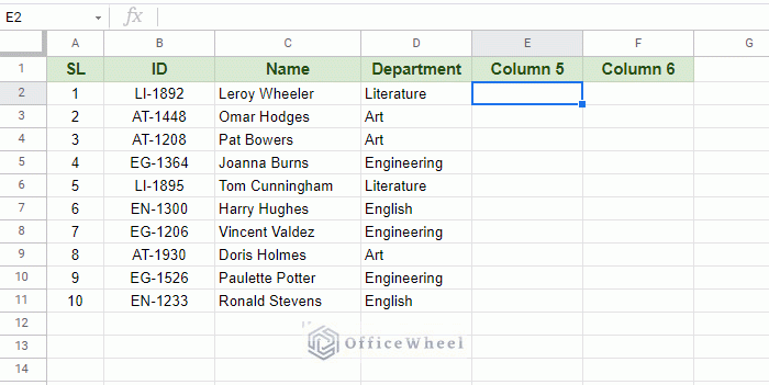
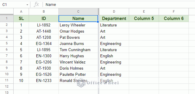
Our result:
Can you freeze columns on merged cells?
No. You can’t freeze columns that contain cells that are merged. You will be hit with the following warning when you look to do so:
Read More: How to Freeze Panes in Google Sheets (3 Simple Ways)
2. Freeze Columns Using the Options Menu in Google Sheets
The traditional way to freeze columns is to do so from the Tab/Options menu. Namely the View tab.
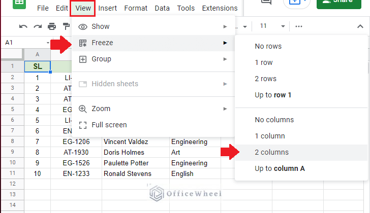
View tab > Freeze > Column
In the Columns section (the second half of the Freeze option) we can see a few options presented to us.
By default, options 1 column and 2 columns are presented to us, allowing us to freeze up to the first two columns.
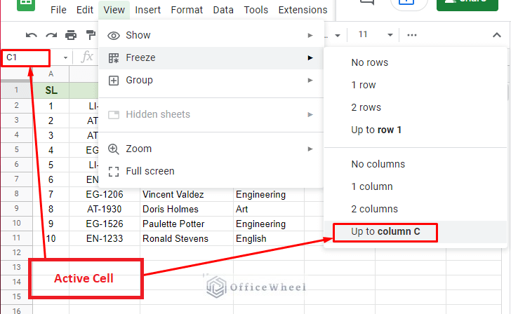
The final option, however, depends on your active cell (Up to column A). In the image, our active cell was A1.
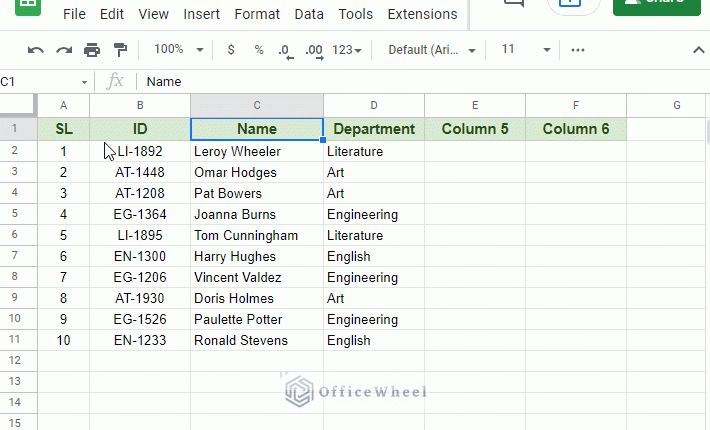
Let’s change our active cell to C1 and see our options.
Now, if we select the option Up to column C:
3. Freeze Columns in Google Sheets from a Mobile Device
Google Sheets can also be found as a mobile device application, for both Apple and Android devices.
Let’s look at how we can freeze columns in Google Sheets using a mobile device.
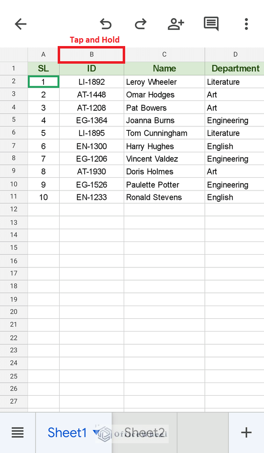
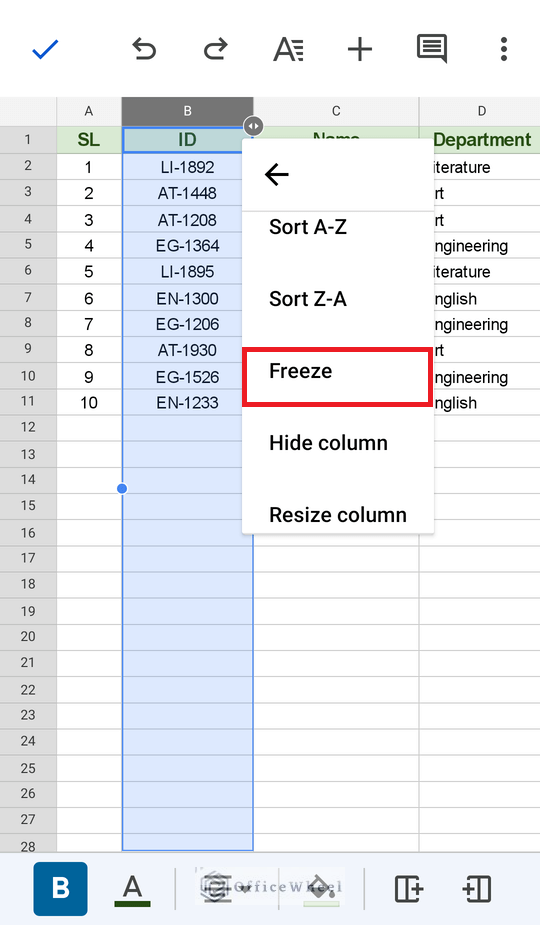
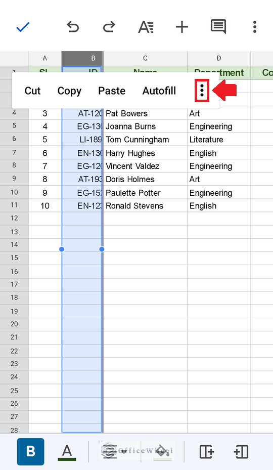
Step 1: Tap and hold the column header until the whole column is selected and a menu appears.
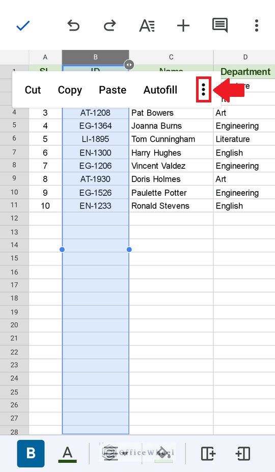
Step 2: Click on the 3-dots icon to open a drop-down menu.
Step 3: Scroll down the drop-down menu to find the Freeze option. Tap it.
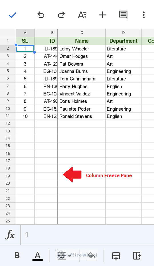
Great! you have successfully frozen two columns from a mobile device.
How to Unfreeze Columns
1. Column Pane
To begin with, unfreezing columns can be done the same way as we have shown in our first method in Google Sheets. That is by dragging the Column pane.
2. View Tab
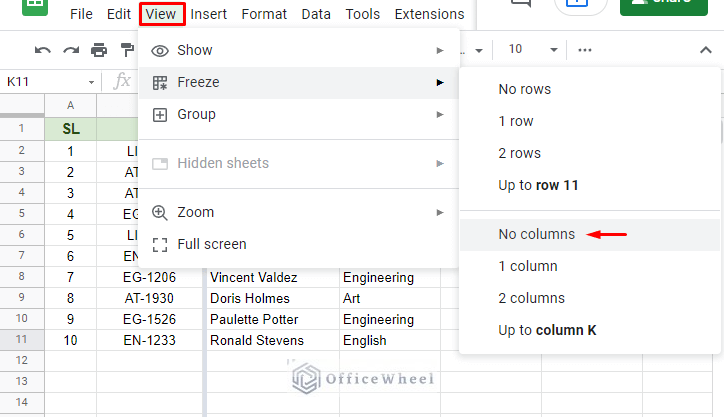
You can also unfreeze your columns by using the View tab
View tab > Freeze > No columns
3. Mobile Devices
In this example, we will be looking at how to unfreeze columns on an Android device.
Step 1: Tap and hold the heading of the column until a tray of options appears.
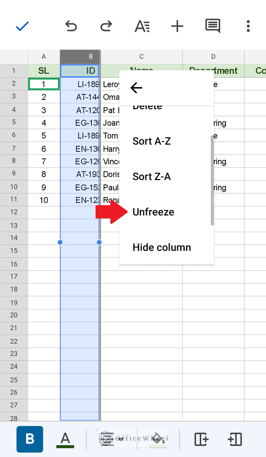
Step 2: Here, click on the 3-dots icon to open a drop-down menu.
Step 3: In the drop-down menu, scroll down to find the Unfreeze option. Select it.
Final Words
We hope that all the methods we have discussed come in handy when you look to freeze, or unfreeze, columns in your Google Sheets spreadsheet.

