Google Sheets has improved in functionality by quite a bit over the years. We now have not only one but two different ways we can filter data if it contains a value in Google Sheets.
First is the traditional filter, which now contains a plethora of different default options that seemingly covers any condition that the user might throw at it.
The second is the FILTER function, which works similarly to the regular filter but in the function form. Meaning that its potential for filter customizations is virtually endless!
Let’s see how we can utilize each option to work with the topic of the day.
How to Filter Data if it Contains Value in Google Sheets
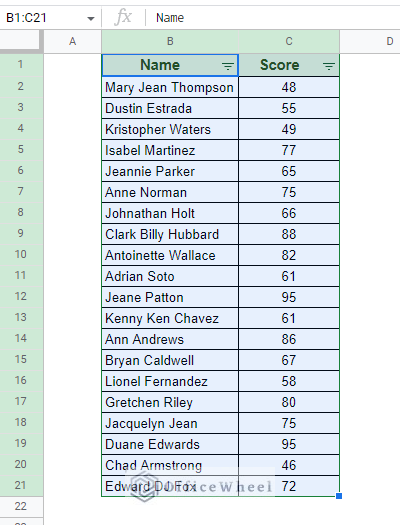
For this section, we will use the traditional filter of Google Sheets. For the following examples, we have created a dataset and applied a filter to it:
1. Filter Data if it Contains Text in Google Sheets (Includes Partial Text Match)
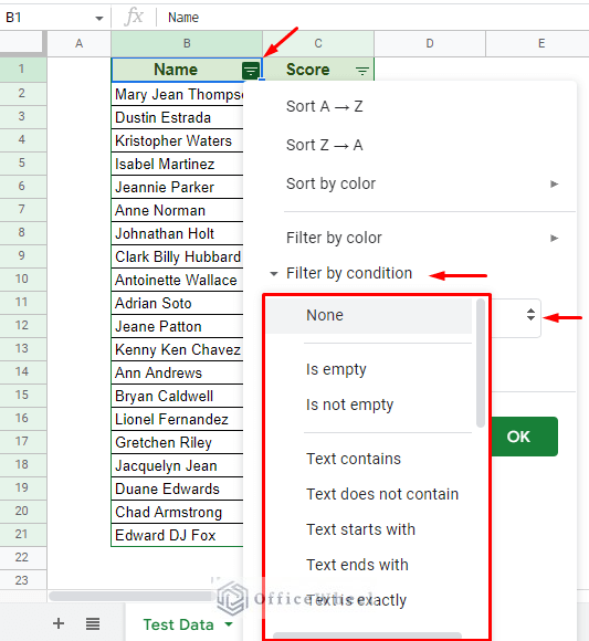
As we have mentioned before, the most used filter conditions can be found in the traditional filter itself. More precisely, in the Filter by condition menu:
Filter > Filter by condition > Drop-down menu
As you can see right at the top, there are already several text-related filter conditions. We can utilize these options to filter data if it contains specific text values in Google Sheets.
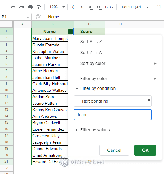
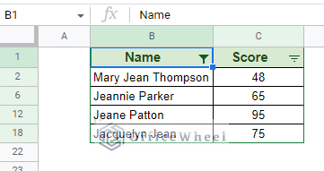
For this example, we will filter all entries that contain the text “Jean” in our dataset.
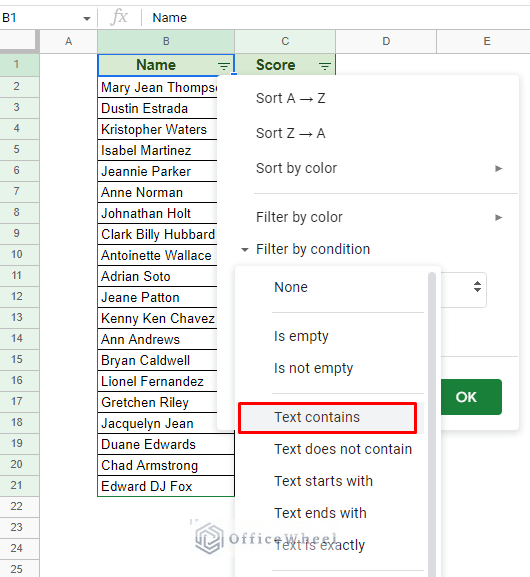
Step 1: Select the “Text contains” option from the Filter by condition section of the filter. “Text contains” searches for the given text within the cells and returns all matching instances.
Step 2: Enter the desired text. In our case, it is ‘Jean’.
Step 3: Click OK to apply.
Alternative: Using a Custom Formula
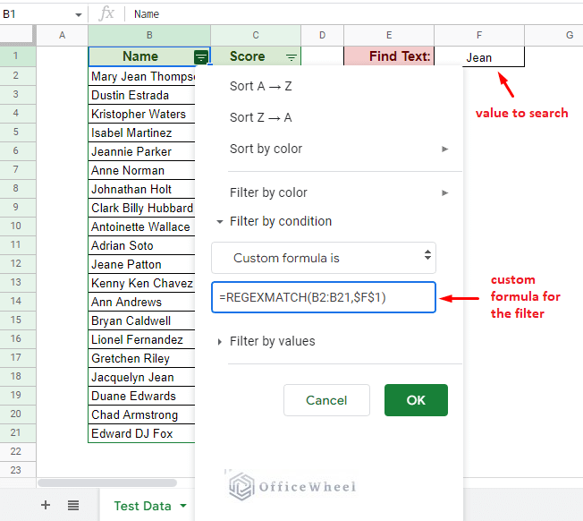
Instead of putting the name down in the filter every time, we can dynamically reference a cell that contains the name to filter the data in Google Sheets.
For that, we have to use a custom formula in the filter. And to match text, we must use the REGEXMATCH function to incorporate regular expressions.
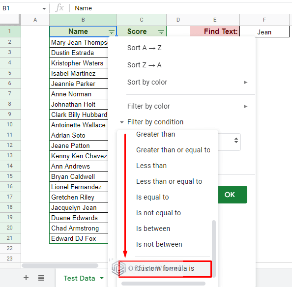
Step 1: To apply a custom formula, scroll down the Filter by condition menu to find the “Custom formula is” option.
Step 2: Enter the following custom formula:
=REGEXMATCH(B2:B21,$F$1)Note: We have used absolute cell reference ($) for the search value (cell F1) to lock the cell reference for the data range.
Step 3: Click OK to apply.
Learn More: How to Filter Custom Formula in Google Sheets (3 Easy Examples)
As you can see, both methods include partial text matches as well.
On top of that, these approaches are also case insensitive. Depending on the scenario, this can be considered an advantage or a disadvantage.
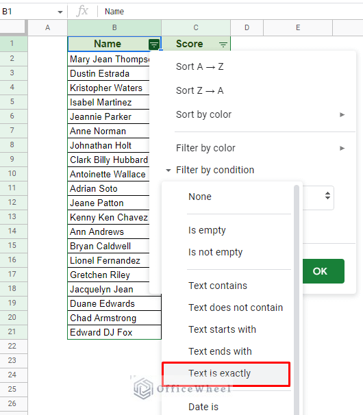
However, if you want a case-sensitive filter, there is always the “Text is exactly” option.
2. Filter if Data does not Contain Value in Google Sheets
Filtering data that does not contain a value in Google Sheets follows similar principles as filtering data that do.
Let’s say we want to find all data entries that do not contain a text or a partial text, which in this case is “Jean”.
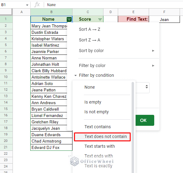
We can once again find the perfect option right in the filter menu under the Filter by condition section. This is the “Text does not contain” option.
Filter > Filter by condition > Text does not contain
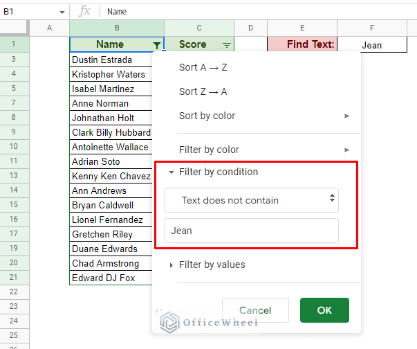
Enter the text “Jean” and press OK to filter the dataset to show all entries that do not contain the text.
Alternative: Using a Custom formula to Filter Data that does not Contain Text
Like before, we can also implement a custom formula to filter entries that do not contain a value in Google Sheets.
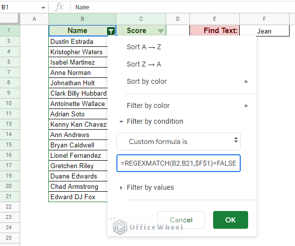
And like before, we must enter the formula under the “Custom formula is” option in the filter.
Filter > Filter by condition > Custom formula is
Of course, we have to modify the formula to satisfy the requirements. The new formula is:
=REGEXMATCH(B2:B21,$F$1)=FALSEThe FALSE condition added to the end of the formula simply gives us the opposite result to “contains text”.
3. Filter Contains Multiple Criteria in Google Sheets (Text Starts With)
Oftentimes we may be asked to filter with multiple conditions.
For example, let’s say that on top of finding all entries with “Jean” we also want to find all entries that start with the letter “A”.
Both conditions are valid and are possible to achieve individually.
Unfortunately, the traditional filter does not have an option to work with multiple criteria. Yet.
But worry not! Where the default options fail, the custom formula succeeds.
Thanks to formulas being so flexible in Google Sheets, we can customize our existing REGEXMATCH formula to take in multiple conditions.
Let’s see the process step-by-step:
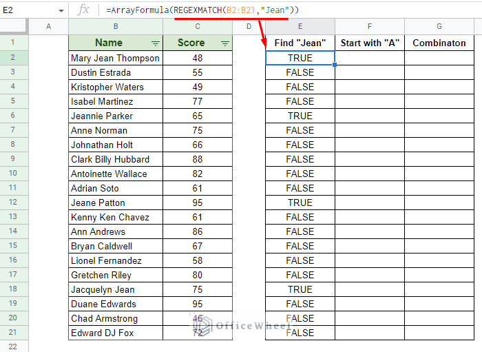
Step 1: Here we have the original formula that we used to find and filter the text “Jean” previously. This shows how Google Sheets views our formula and how it is used in the filter.
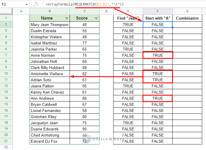
REGEXMATCH(B2:B21,"Jean")Step 2: We use the same principles to create a regular expression formula to satisfy the condition “text starts with A”. The regular expression of the symbol that determines the starting point of a text is “^”.
Thus, the formula is:
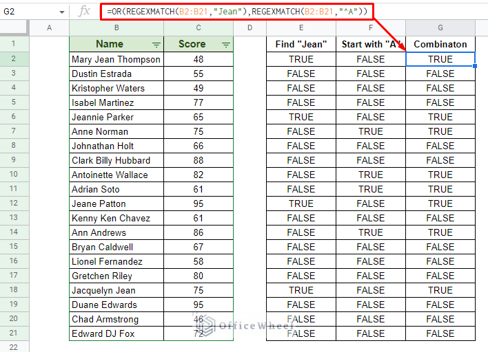
REGEXMATCH(B2:B21,"^A")Step 3: Combine the two formulas following the “Or” condition. Thankfully, we have the OR function ready and available.
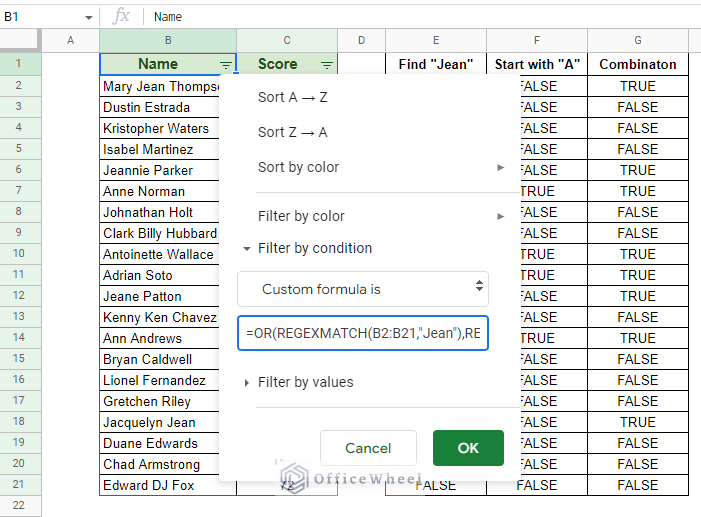
=OR(REGEXMATCH(B2:B21,"Jean"),REGEXMATCH(B2:B21,"^A"))This is the custom formula we will use for the filter.
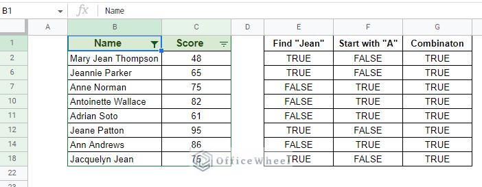
Step 4: Input this formula in the custom formula field of the filter. Click OK to apply.
The result:
Using the FILTER Function to Filter Values if it Contains Specific Value in Google Sheets
The FILTER function is a great way to approach filtering in Google Sheets. This is because, on top of preserving the source data, it has all the advantages of a function’s features in a spreadsheet.
FILTER function syntax:
FILTER(range, condition1, [condition2, ...])Using the FILTER function is much like working with custom formulas for filters, only this time, the results are shown separately.
Let’s see how we can use this function to filter data that contains text in Google Sheets.
1. Filter Data Containing a Single Text
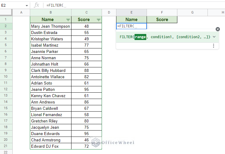
Step 1: Open a FILTER function in any cell of the worksheet. An advantage of using formulas is that we can present the results in the same or different worksheets.
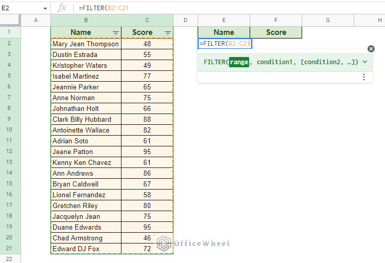
Step 2: Select the data range for the function.
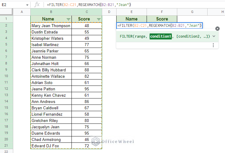
Step 3: Input the filter criteria. Like in custom formulas, we will once again use REGEXMATCH to find the text criteria from the data source. We can simply put in the same formula:
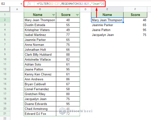
Step 4: Close parentheses and press ENTER.
=FILTER(B2:C21,REGEXMATCH(B2:B21,"Jean"))2. Filter Data Containing Multiple Texts
It is when we have multiple criteria, we need to rethink our original approach.
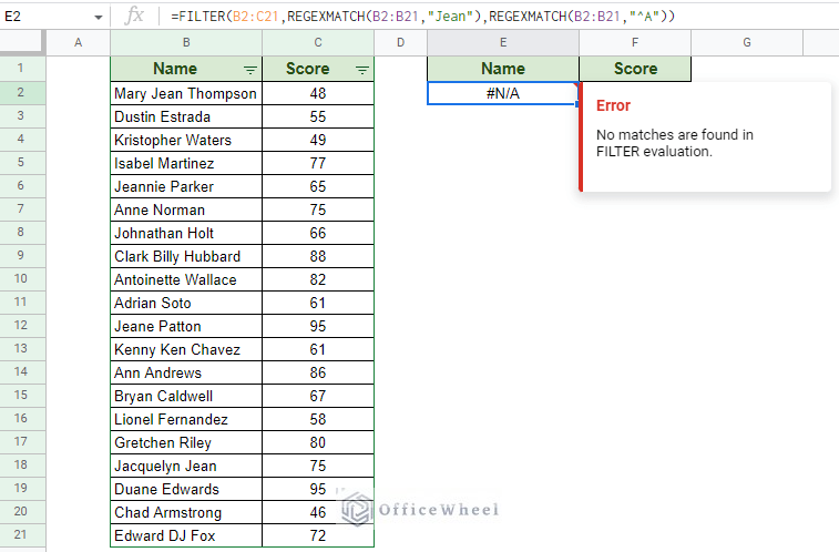
The multiple conditions that the FILTER function allows us is in the AND logic. So, putting different regular expression matches as conditions will not work for the OR criteria.
- Has text “Jean” OR starts with “A”: Will not work
- Has text “Jean” AND starts with “A”: Will work
So, we must take a different approach. Luckily, regular expressions are quite versatile. We can use the OR argument for regular expressions within the first REGEXMATCH function.
The symbol for regular expression OR condition is “|”.
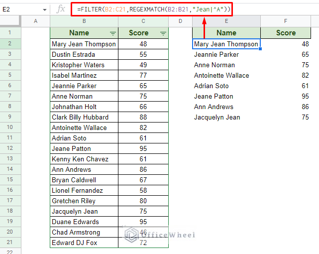
So, if we want to filter data that either contains the text “Jean” or if the value starts with “A”, the filter formula will be:
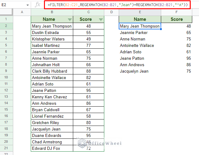
=FILTER(B2:C21,REGEXMATCH(B2:B21,"Jean|^A"))Alternatively, you can also use the plus (+) symbol to implement the OR condition:
=FILTER(B2:C21,REGEXMATCH(B2:B21,"Jean")+REGEXMATCH(B2:B21,"^A"))Final Words
That concludes our simple guide on how to filter data if it contains a value in Google Sheets.
Using either traditional filters or FILTER formulas has its own advantages and disadvantages. But in both cases, custom formulas give more freedom to the users to exactly filter as required.
Feel free to leave any queries or advice you might have in the comments section below.

