Today, we will look at a few ways we can count days from a date to today in Google Sheets. While there are multiple ways to go about it, some may be suited to certain situations more than others. But first, let’s start with some basic understanding.
Understanding How to Calculate Days Between Dates in Google Sheets
Before we get into our main topic for the day, we must first understand how basic date calculations, like finding the number of days, work in Google Sheets. You can, of course, skip ahead to the meat of the article.
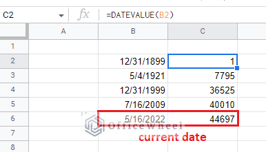
Primarily, Google Sheets views date as an integer value, starting from 12/31/1899 which has a value of 1 (this is the first noted date in Google Sheets). While today’s date, which is 5/16/2022 at the time of writing, has a value of 44697. These date values can be easily extracted by using the DATEVALUE function.
What this means is that every single day has its own integer value. This makes day calculations that much easier.
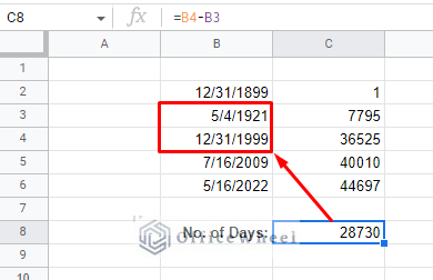
For example, if we want to count the number of days between the 2nd and 3rd days in our list, we simply have to perform an arithmetic subtraction:
=B4-B3This is the fundamental approach to counting days in Google Sheets. The rest of the article discusses this and other practical alternatives for counting days based on criteria.
5 Ways to Count Days from Date to Today in Google Sheets
1. Use Simple Arithmetic Subtraction to Count Days in Google Sheets
Since we are calculating from a date to today, it is best to use the TODAY function to generate the current date automatically.
The date generated by TODAY is “running”, meaning that every time the worksheet is refreshed the date will be updated to the latest value. On the downside, however, too many TODAY functions can overwhelm the worksheet. But we have a solution to that later in this section.
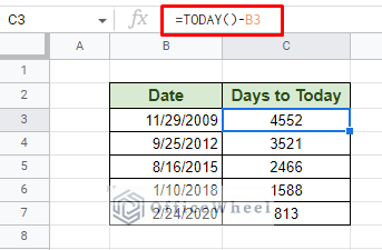
So, to count the number of days from a date to today in Google Sheets using simple arithmetic subtraction, our formula is:
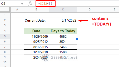
=TODAY()-B3As you have noticed, every single row has a TODAY function in it for calculation. This recurring calculation puts a lot of stress on the application. To remedy this, we will put the TODAY function in a separate cell and pull that data with an absolute cell reference to use in our formula.
=$C$2-B52. Using the MINUS Function
The direct substitute for simple arithmetic subtraction is the MINUS function of Google Sheets. Its application is as easy.
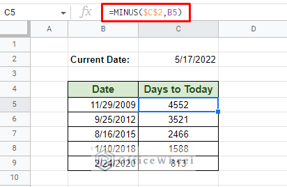
=MINUS(end_date,start_date)This makes our formula:
=MINUS($C$2,B5)Alternatively, with the TODAY function within the formula:
=MINUS(TODAY(),B5)3. Using the DAYS Function
The DAYS function was explicitly created to count the number of days between two dates.
DAYS(end_date,start_date)It is a lot like the MINUS function and can factor in any leap year days.
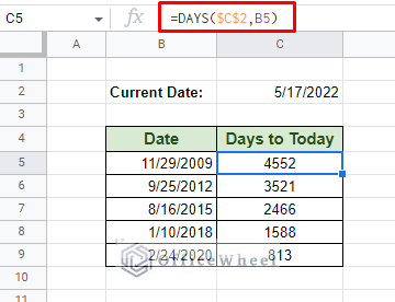
The DAYS function in action to count the number of days from a date to today in Google Sheets:
=DAYS($C$2,B5)The DAYS function with TODAY:
=DAYS(TODAY(),B5)4. Using the DATEDIF Function
The DATEDIF function is one of the more useful date functions of Google Sheets. It not only finds the difference between two dates but does so in the type of value that the user needs. Be it days, months, years, and more.
DATEDIF(start_date, end_date, unit)Since we are only working with days, we will leave the unit field with just “D”. Also notice that for the first time, we have the start_date before the end_date as a field. It is a good thing to keep this arrangement in mind to avoid errors.
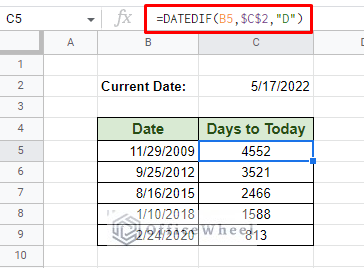
So, to count the number of days from a date to today in Google Sheets, our formula with DATEDIF will look like this:
=DATEDIF(B5,$C$2,"D")DATEDIF with the TODAY function within it:
Learn More: Use DATEDIF from Today in Google Sheets (An Easy Guide)
5. How Do I Count Workdays to Today in Google Sheets?
So far, we have counted all 7 days of the week between two dates in our spreadsheet. But, in a professional setting, it is not uncommon to calculate only the workdays or business days of an organization.
Again, Google Sheets provides us with the perfect function for such a calculation, that is the NETWORKDAYS function.
NETWORKDAYS(start_date, end_date, [holidays])The function treats Saturdays and Sundays as weekends, meaning that these two days are not considered in the count.
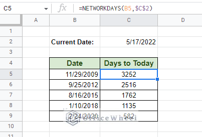
So, counting the number of workdays from a date to today in Google Sheets:
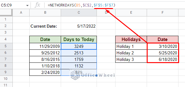
=NETWORKDAYS(B5,$C$2)As you may have noticed, further allows the user to add holidays to ignore in the date count. The best way to do this is to add a separate table that lists all the holidays to include. Later, add that range of cells in the [holidays] field.
=NETWORKDAYS(B5,$C$2,$F$5:$F$7)On the other hand, if Saturdays and Sundays are not the weekends in your organization or region, you can always opt for NETWORKDAYS.INTL function to manually input the weekend combination that suits your data.
Point to Note about Date Functions in Google Sheets
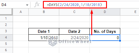
Date functions like the ones we have used in this article: DAYS, DATEDIF, and NETWORKDAYS, cannot take a date directly into their fields. We get an error if we do so as you can see in the following image:
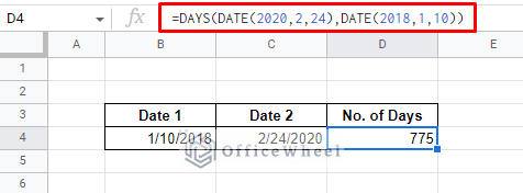
So, you have to either reference the cells containing dates as we have done in our article or use the DATE function to input the date value in the fields.
Final Words
That concludes all the ways we can count days from date to today in Google Sheets. While the calculation can be done with simple arithmetic subtraction, it is always a better idea to take advantage of the date functions that Google Sheets has on offer.
Feel free to leave any queries or advice you might have for us in the comments section below. Or have a look at some of our other date-related articles.

