Use DATEDIF from Today in Google Sheets (An Easy Guide)

We can approach how we can find the difference in date in Google Sheets in multiple different ways. But perhaps the best way is to use the DATEDIF function. So today, we will show you how to use DATEDIF from today in Google Sheets to better present our argument.

Let’s get started.

What is the DATEDIF function of Google Sheets?

Simply put, we can calculate the difference between two dates using the DATEDIF function. The advantage of using this function is that the user can determine the type of output that is presented. Where a simple arithmetic date calculation gives the date difference in days by default, DATEDIF can present the difference in days, months, and years.

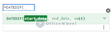
Let’s bring our attention to the unit field of the function. This field takes characters corresponding to the type of output the user requires. They are:

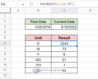
• “D”: Gives the total number of days between the start date and end date.
• “M”: Gives the total number of whole months between the start date and end date.
• “Y”: Gives the total number of whole years between the start date and end date.
• “MD”: Gives the number of days between the start date and end date without counting the months or years completed.
• “YM”: Gives the number of whole months between the start date and end date without counting the months and years completed.
• “YD”: Gives the number of days between the start date and end date, assuming that the date range is no more than one year apart.

As you can see, using the DATEDIF function is easy:

• Open the DATEDIF function in a cell, =DATEDIF(.
• Reference the cell that contains the start_date, usually the date that is previous or the past.
• Reference the cell that contains the end_date, usually the date that comes after.
• Type in one of the units in quotations to determine the output result.
• Close parentheses and press ENTER.

Simpler Alternative: Find the Number of Days ONLY

If you are only looking to find the number of days, we have a couple of simpler alternatives for you. Since each date in Google Sheets holds an integer value, we can find the difference of days between two dates using simple arithmetic subtraction.

OR

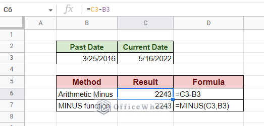
But for month and year date differences, it is best to use DATEDIF or a combination of other date functions of Google Sheets.

Using the DATEDIF function with Today in Google Sheets

How to get today’s date in Google Sheets?

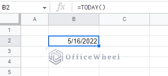
Google Sheets provides us with a simple way to generate today’s date or current date in a worksheet, that is by using the TODAY function.

Features:

• A standalone function that takes no parameters.
• Returns a “running” date. The date updates every time the worksheet is refreshed or opened. (You can change this feature in settings. File > Settings > Calculation > Recalculation)

Using the TODAY function with DATEDIF, we can calculate the date difference between the current date and another date.

Calculate Date Difference with DATEDIF from the Current Date

We have already seen how to implement the DATEDIF function and seen how to find the difference between dates in days.

But, as a refresher, here is the formula to calculate the number of days from date to today:

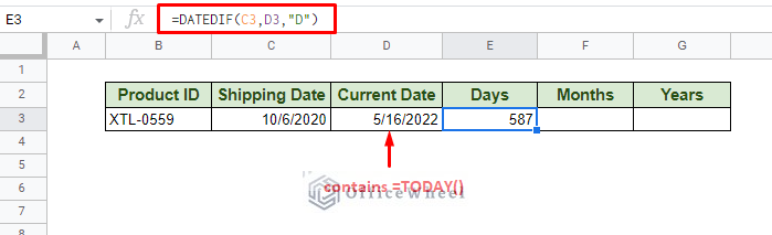
The key input over here is the “D” which tells the function to return our result in terms of days. This is essentially subtracting the Shipping Date from the Current Date (Today).

The Current Date cell contains the TODAY function. Alternatively, you can directly use the TODAY function inside the DATEDIF function.

Calculate Difference in Months from Today in Google Sheets

Similarly, we can calculate the number of months from a date to the current day with DATEDIF. The only update will be the unit field with “M” for the month calculation.

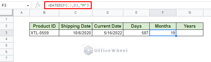
If you want to use the TODAY function within DATEDIF:

Learn More: How to Subtract Months from Date in Google Sheets (3 Easy Ways)

Calculate the Number of Years from Today

To calculate in terms of years, we simply change the unit field to “Y”, keeping the rest of the formula the same:

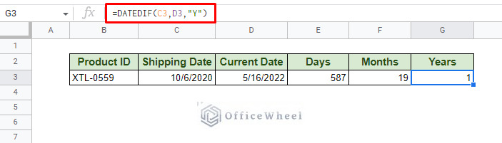
Note that the calculation for both months and years returns the number of completed months and years. That is why we get a difference of 1 year between the Shipping Date and the Current Date since 24 months (2 years) have not been completed.

Calculate Tenure in Google Sheets

One of the best practical uses of date difference, especially till the current date, is to calculate the tenure of employees.

The DATEDIF function provides the perfect solution for any manager in this case.

Here we have a dataset of employees with their Join Dates and the dates of their end of employment, with the first two End Dates containing the current dates since they are continuing employees:

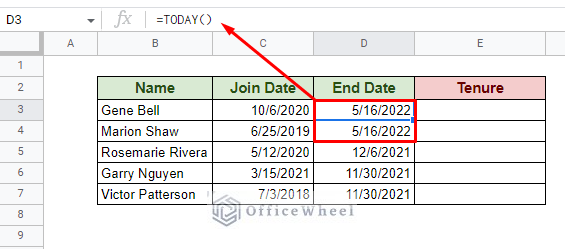
Previously, for long-term employment, tenure was usually calculated in years. For this, you can simply use the unit “Y”.

But we want to go for a more practical approach. We want to make our results more presentable, thus, we get a little creative with our formula.

Calculating tenure of employees in terms of years and months:

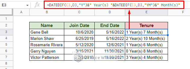
The year calculation, DATEDIF(C3,D3,"Y"),you already understand. So, let’s bring our attention to the month calculation, DATEDIF(C3,D3,"YM").

With unit “M” we would have gotten the total number of months from the start date to the end date. But with unit “YM”, we calculate the number of months after a solid number of years has passed.

And it is thanks to this versatility, we can output a practical result for the total time elapsed.

We have also added some flavor text which we concatenated with the formula using an ampersand (&).

Similarly, if we want to include the number of days elapsed into our result, our formula will look like:

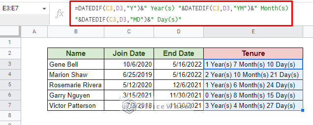
Learn More: How to Calculate Tenure in Google Sheets (An Easy Guide)

Final Words

That brings us to the end of our discussion of how we can use DATEDIF from today in Google Sheets. The main reason why we use DATEDIF to calculate date differences is its versatility. We can output the difference in multiple ways, including months and years.

Feel free to leave any queries or advice you might have for us in the comment section below. Or have a look at some of our other date-related articles that are sure to interest you.

Related Articles for Reading

• Find and Display Current Date in Google Sheets (Easy Guide)
• How to Subtract Dates in Google Sheets (An Easy Guide)
• Add 7 Days to Date in Google Sheets (And More)
• How to Organize Google Sheets by Date (3 Easy Ways)
• How to Add Months to a Date in Google Sheets (2 Easy Ways)