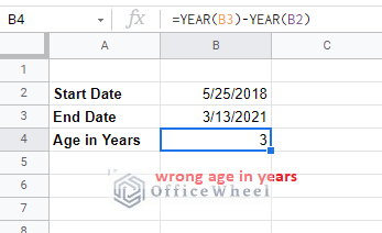
How to Calculate Tenure in Google Sheets (An Easy Guide)

A common misunderstanding that many new users of spreadsheets have is how age is calculated. One might think that a simple subtraction will get the work done.

While subtraction between years can be done, Google Sheets will not consider the months into account. This means that by subtracting dates, let’s say between 5/25/2018 and 3/13/2021, Google sheets will return a 3-year difference, even though 3 years have not passed.

So, in this article, we’ll show you how to properly calculate the age, more specifically the age of service or tenure in Google Sheets.

Let’s get started.

Table of Contents

How to Calculate Tenure in Google Sheets

Calculate Tenure in Years (or Years of Service) in Google Sheets

The easiest way to calculate date-related differences is to use the DATEDIF function.

The DATEDIF function syntax:

DATEDIF(start_date, end_date, unit)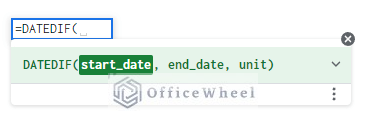

As you can see, the input fields are quite easy to understand. So, I bring your attention to the unit field. Here, you can input the type of output you desire: Days, Months, or Years.

Here is a list of what inputs the unit field takes:

“Y”: Gives the total number of whole years between the start date and end date.
“M”: Gives the total number of whole months between the start date and end date.
“D”: Gives the total number of days between the start date and end date.
“MD”: Gives the number of days between the start date and end date without counting the months or years completed.
“YM”: Gives the number of whole months between the start date and end date without counting the months and years completed.
“YD”: Gives the number of days between the start date and end date, assuming that the date range is no more than one year apart.

Thus, our formula to calculate age or tenure in years will be:

=DATEDIF(B2,B3,"Y")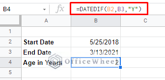

For a more practical scenario we have created the following dataset:

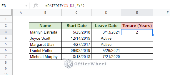
The first tenure is already calculated, but what to do for “Active” employees?

Active means that they are currently employed, thus we calculate our end date to be today. Which can be represented by the TODAY function.

=DATEDIF(C4,TODAY(),"Y")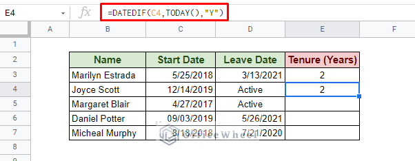

But having two different functions in a single column is not intuitive nor is it a good idea. So, we have created a universal formula that can be applied to the whole column with the help of the IF function.

=IF(D3="Active",(DATEDIF(C3,TODAY(),"Y")),(DATEDIF(C3,D3,"Y")))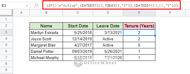

Alternative: The YEARFRAC Function

The YEARFRAC function returns the number of years between two dates in Google Sheets. The fact that it can also return fractional years will be useful to calculate tenure in Google Sheets.

On its own, the YEARFRAC function gives is the following result:

=YEARFRAC(B2,B3)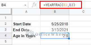

$tenure in fractional years$

It did give us the years, but in fractions/decimals. To get an integer year tenure, we must enclose the formula in the INT function.

=INT(YEARFRAC(B2,B3))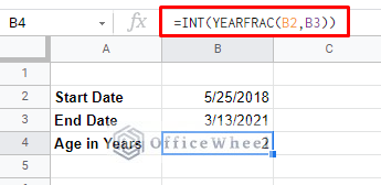

$how to calculate tenure in years in google sheets using the yearfrac function$

Practical dataset: Calculate tenure in years in Google Sheets using YEARFRAC function:

=IF(D3="Active",INT(YEARFRAC(C3,TODAY())),INT(YEARFRAC(C3,D3)))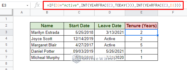

$using yearfrac to calculate tenure in a practical setting$

Calculate Tenure or Age of Service in Years and Months in Google Sheets

In a professional setting, it is better to present the tenure of an employee not only in years but also in months covered.

Recall our list of units for the DATEDIF function. The “YM” unit will present us with the current number of months covered in the running year.

DATEDIF(start_date,end_date,"YM")

Unfortunately, we hit another snag at this point. The DATEDIF function cannot output both the year and month data simultaneously. We have to put the two separate outputs in a single cell for presentation.

So, our formula looks something like this:

=DATEDIF(C3,D3,"Y")&" Year(s) and "&DATEDIF(C3,D3,"YM")&" Month(s)"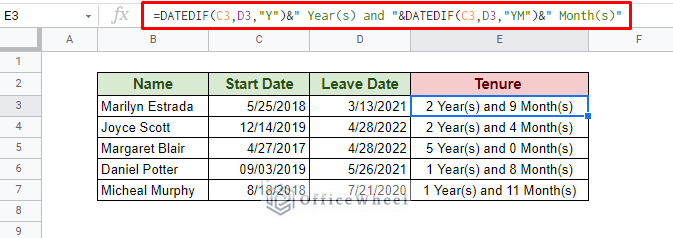

Using ampersand (&) we were able to concatenate the two results of DATEDIF into one cell to a more professional-looking outcome.

Extra: Calculate Tenure in Years, Months, and Days

Why not go a step further and add the number of covered days while we are at it?

Since we are looking for the number of days after a month is completed, the unit field will have “MD”.

Our formula:

=DATEDIF(C3,D3,"Y")&" Year(s) and "&DATEDIF(C3,D3,"YM")&" Month(s) "&DATEDIF(C3,D3,"MD")&" Day(s)"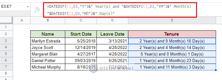

Final Words

Calculating tenure in Google Sheets is quite simple as you have seen in this article. Only that you have to use a date function like DATEDIF to get the job done. Regula arithmetic functions like minus will not work correctly with dates.

Feel free to leave any queries or advice you might have in the comments section below. Or go ahead and have a look at our other date-related articles to make your Google Sheets experience simpler.