Adding values under certain conditions is a common affair in Google Sheets. But one approach that can be used to simplify a condition is the checkbox. As such, today we will look at how we can sum values if checked in Google Sheets.
Let’s get started.
2 Ways to Sum Values If Checked in Google Sheets
1. Using the SUMIF Function
For our first method, we look to the SUMIF function. The function is highly intuitive for this problem since it does exactly what we want: sum according to a condition.
The SUMIF function syntax:
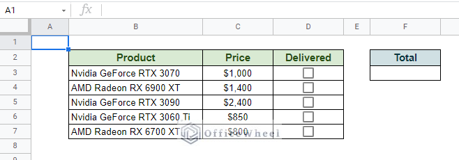
SUMIF(range, criterion, [sum_range])We will utilize all three of the fields for the following dataset to calculate the total per the checked Delivered boxes:
Let’s go through the process step-by-step.
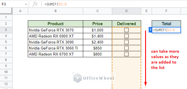
Step 1: Open the SUMIF function in the target cell and input the criterion range. To future-proof the formula, we have removed the column range limitation. We use D3:D instead of D3:D5.
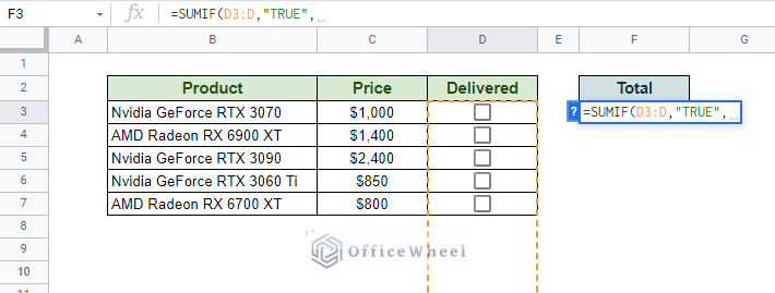
Step 2: Add the criterion. A checked checkbox means that its value is TRUE. Thus, our criterion will be “TRUE”.
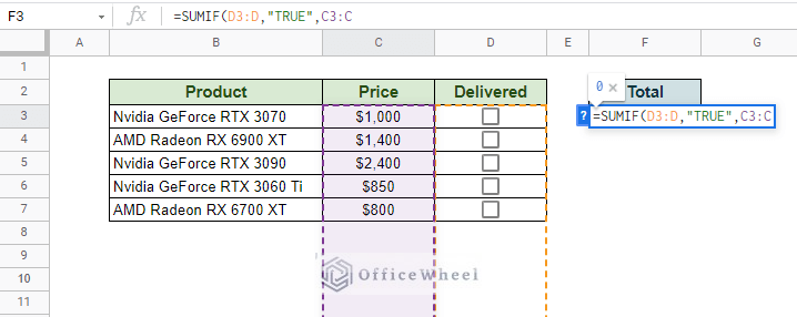
Step 3: Input the sum range. This will be our Price column. Same as the criterion range, we are keeping the sum range open-ended, C3:C.
Step 4: Close parentheses and press ENTER.
=SUMIF(D3:D,"TRUE",C3:C)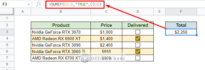
Note: We have applied conditional formatting to our dataset to highlight our choices. To know more about how we achieved this, please see our Conditional Formatting with Checkbox in Google Sheets article.
2. Using the SUMPRODUCT Function
Our next method revolves around the SUMPRODUCT function. Since the function is versatile, it can easily mimic the idea and functionality of the SUMIF function.
The SUMPRODUCT function syntax:
SUMPRODUCT(array1, [array2, ...])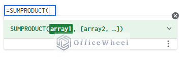
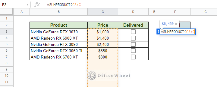
Step 1: We start by opening our SUMPRODUCT function in the target cell and adding the column range of Price. We will keep the range open-ended, C3:C.
Step 2: Input the AND operator or the asterisk (*) symbol.
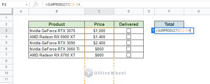
What this does is that it applies the AND logic to the statement to check whether both cells in each row have positive values, aka TRUE:
- The Price column will always be TRUE since it contains a numerical value.
- The checkbox only returns TRUE when it is checked.
So, when the checkbox is TRUE, the function will return the Price to the calculation as it satisfies a positive AND logic (TRUE and TRUE).
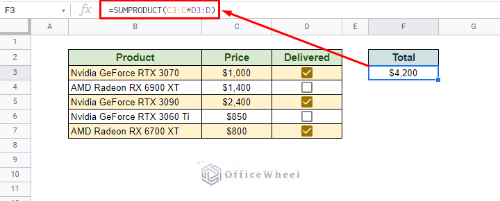
Step 3: Input the range of the Delivered column. This too shall be open-ended, D3:D.
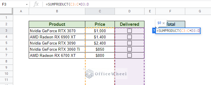
Step 4: Close parentheses and press ENTER.
Final Words
That concludes all the ways we can use to sum values depending on checked conditions in Google Sheets. While the SUMIF function may be more intuitive and a simpler solution to this problem, the SUMPRODUCT function can prove to be more worthwhile to know for different scenarios.
Please feel free to leave any queries or advice you might have for us in the comments section below.