In this article, we will discuss how to sum the duration of time in Google Sheets. At first glance, the idea may seem simple, but a certain level of understanding of data types is involved to fully utilize the methods we will discuss here.
Let’s dive in.
2 Ways to Sum a Duration of Time in Google Sheets
1. Using Simple Addition to Calculate the Total Duration
There are many instances where the sum of a duration of time is required. Let’s take this employee workday duration for example:
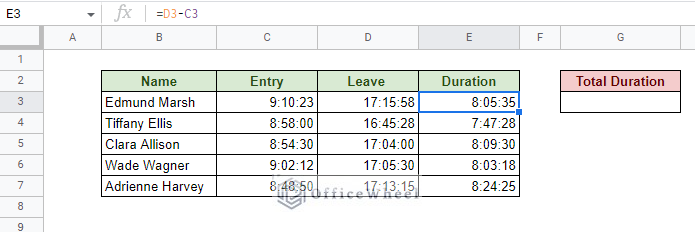
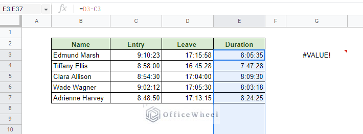
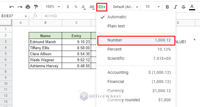
Calculating the duration from Time A to Time B is a matter of subtracting the time values (D3-C3).
So, finding the total duration of effective work hours can be simply done by adding the durations together, right?
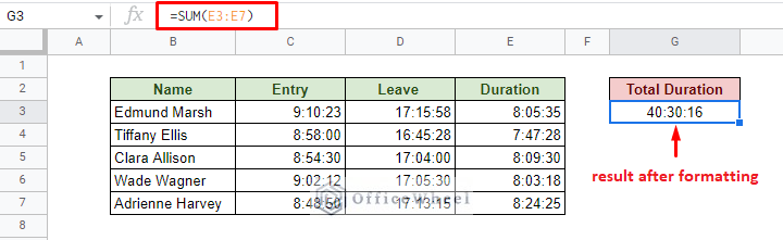
Let’s see what happens when we apply the SUM function to find the total duration of time in Google Sheets:
=SUM(E3:E7)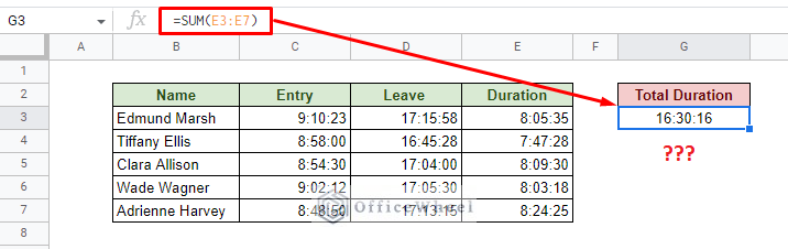
That doesn’t look right, does it?
The sum of the duration should have been at least 40 hours, but the result of the SUM function is only showing 16 hours and 30 minutes.
Why is that?
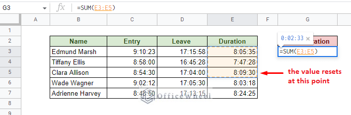
The Problem with the SUM function when calculating Time (The 24 Hour Limit)
In Google Sheets, functions like SUM take on the base value type of its arguments, which in this case was time.
We all know that the time format type has a limit of 24 hours according to the 24-hour clock. So, when using time values in the SUM function will limit the calculation to 24 hours (or 00:00:00) after which the clock resets and the value repeats.
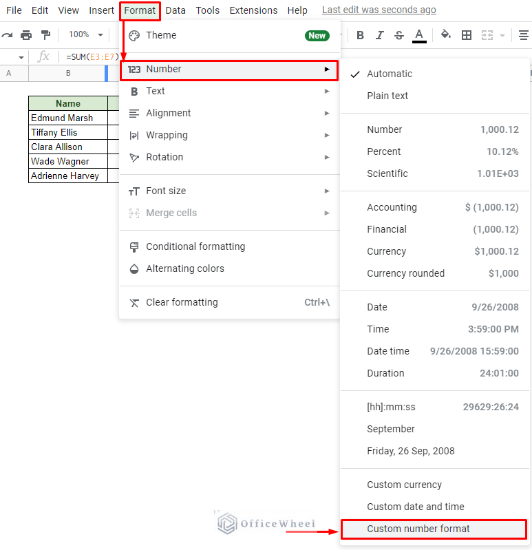
Solution 1: Changing the Number Format
The easiest solution to this problem is changing the format of time itself. By default, no time format in Google Sheets accommodates for more than 24-hour calculation. So why not create a custom time format ourselves?
Step 1: Select the cell you want the format changed, for us, it’s cell G3, and navigate to the “Custom number format” option from the Format tab.
Format > Number > Custom number format
Step 2: Type in the following time format:
[hh]:mm:ss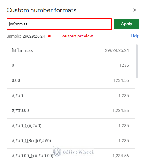
The square braces [] removes the 24-hour limitation from the hour value.
Step 3: Click APPLY to apply the formatting in the Total Duration cell.
Solution 2: Using TEXT and TIMEVALUE functions
Another way to change the time value format directly is by using the TEXT function. But before we can do that, we must first extract the underlying time value of the sum.
We can do this by applying a combination of the SUM and TIMEVALUE functions:
=ArrayFormula(SUM(TIMEVALUE(E3:E7)))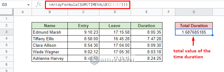
Note: We use the ARRAYFORMULA function around our formula to take into account the range of cells, E3:E7, that contain time duration.
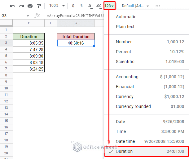
And now, we can either change the format of the cell to Duration.
Or, keep it within the realm of functions and use the TEXT function to update the format of the cell:
=ArrayFormula(TEXT(SUM(TIMEVALUE(E3:E7)),"[hh]:mm:ss"))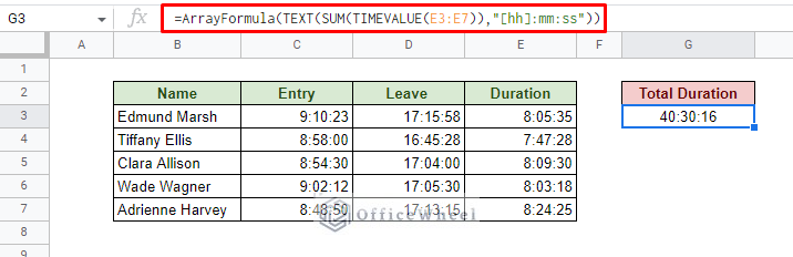
We can take this formula further and make it more dynamic by changing the cell range from E3:E. This will allow the formula to also consider new entries.
However, having a blank cell in this range will cause an error. Therefore, we will also add the IFERROR function to accommodate this.
Our formula:
=ArrayFormula(TEXT(SUM(IFERROR(TIMEVALUE(E3:E))),"[h]:mm:ss"))2. Using QUERY to Sum a Duration of Time in Google Sheets
The QUERY function is perhaps one of the most versatile in Google Sheets. With it, a user can perform almost all kinds of calculations on top of having customized results.
The QUERY function syntax:
QUERY(data, query, [headers])
And we can use this function to sum the duration of time in Google Sheets.
The function is simple, however, there is a catch:
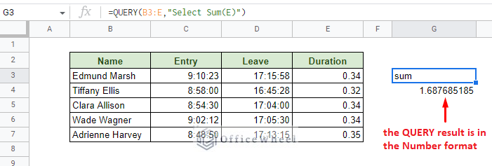
=QUERY(B3:E,"Select Sum(E)")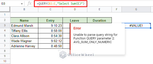
The AVG_SUM_ONLY_NUMERIC error means that the values to sum in column E are not numeric. This is true since they are fundamentally time values. It is a similar problem as we have seen in the previous section of this article.
We can approach this problem in two ways:
- Change the format of column E manually.
- Create a virtual column to convert time to numbers so that QUERY can calculate the values.
I. Change the Time Format to Numbers
The simplest solution to allow the QUERY function to give use the sum of the duration is to convert the Duration column to a Number format.
Step 1: Select the values of the Duration column. It can be E3 to E7 or the entire column starting from E3 (E3:E).
Step 2: Select the Number format from the Toolbar.
We now have a value for our total duration, but it is expectedly also in the Number format.
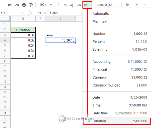
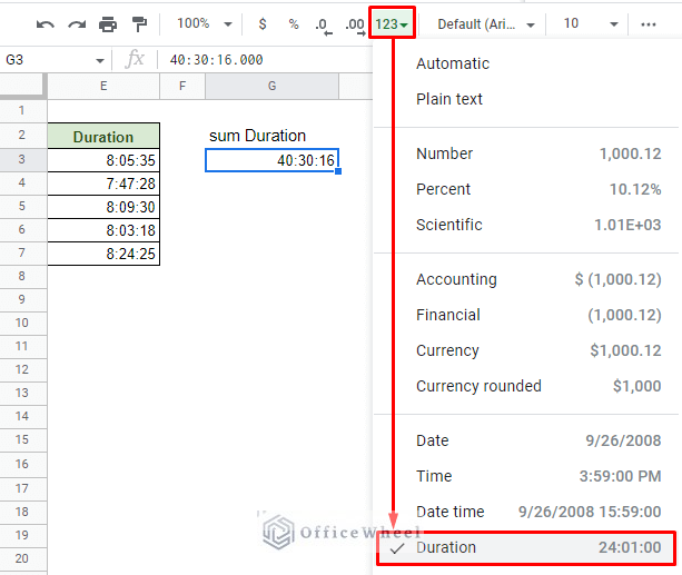
Step 3: Change the QUERY result to the Duration format from the Toolbar.
While using this method is just fine, we’ve sacrificed our Duration column for it.
The next method is a tad more complicated, but it will keep the dataset intact.
II. Using QUERY to Sum Duration without changing the Dataset
Changing the dataset just to accommodate a function may not always be a good idea. So, to use the QUERY function to sum a duration in Google Sheets, we must look at creative approaches to get the right result. We have 3 steps to go through
Steps to Query the Sum of Time Duration
Step 1:
One such way is by creating a virtual column that contains the date in numerical form. We do this by transforming the values of the Duration column into numbers.
The base formula to transform time into numbers:
Hour/24+Minute/1440+Second/86400Applying this formula to the Duration column values to get numerical times:
={"Duration";ArrayFormula(IF(LEN(E3:E),(HOUR(E3:E)/24+MINUTE(E3:E)/1440+SECOND(E3:E)/86400),))}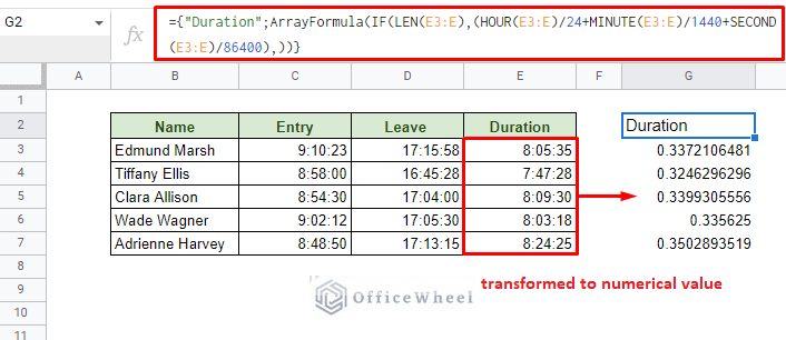
The LEN function is used to control and ignore the blank cells in the range. The ARRAYFORMULA function is used to present all the values in the range.
Step 2:
The next step is to create a data range for the QUERY function. It is usually the dataset, but since we are using the number Duration column, we must create a “virtual” dataset for the function.
The idea is to take the first 3 columns of our dataset, which remain unchanged, and add a fourth column for the new Duration. The syntax:
{B2:D, the virtual Duration column}The formula in action:
={B2:D,{"Duration";ArrayFormula(IF(LEN(E3:E),(HOUR(E3:E)/24+MINUTE(E3:E)/1440+SECOND(E3:E)/86400),))}}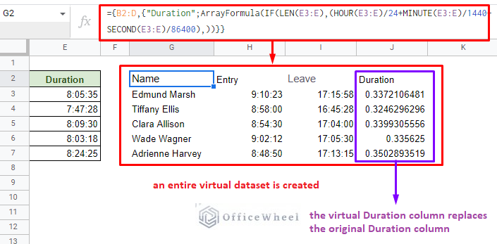
Step 3:
We can now use the virtual dataset within the QUERY function:
=QUERY({B2:D,{"Duration";ArrayFormula(IF(LEN(E3:E),(HOUR(E3:E)/24+MINUTE(E3:E)/1440+SECOND(E3:E)/86400),))}},"Select Sum(Col4)",1)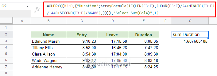
Since we are not using the real column E for our formula, we have put SUM(Col4) instead of Sum(E) for the query argument. Col4 in QUERY points to the 4th column from the start of the dataset, which is the virtual Duration column for our dataset.
Step 4:
We finalize the approach by updating the cell format to Duration from the Toolbar.
Use Case: Find Average Time Duration in Google Sheets
The next step that one can use a summed value for is to find the average. And we are going to do just that with our total duration.
As we understand, the formula is simple:
Sum/Total number of valuesStep 1: For Sum, you can use either of the formulas that we have discussed in this article. We will be using the one with the TIMEVALUE and TEXT formula.
=ArrayFormula(TEXT(SUM(IFERROR(TIMEVALUE(E3:E))), "[h]:mm:ss"))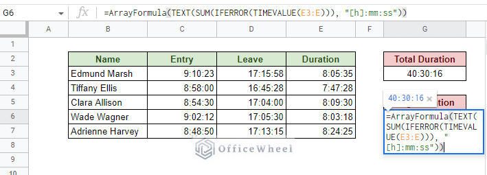
Step 2: For the total number of values, we shall use the COUNTA function with the Duration column as a range. It counts all the cells that have a value.
COUNTA(E3:E)Dividing the Sum with COUNTA:
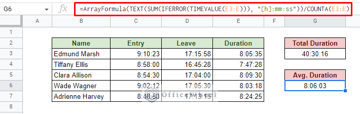
=ArrayFormula(TEXT(SUM(IFERROR(TIMEVALUE(E3:E))), "[h]:mm:ss"))/COUNTA(E3:E)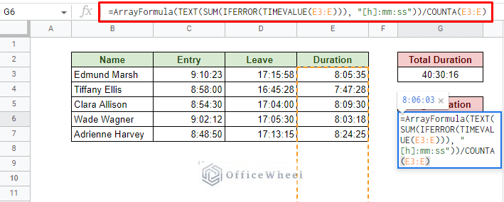
Step 3: Press ENTER to get the result. Update the cell to the Duration format from the Toolbar.
Final Words
That concludes all the ways we can sum the duration of time in Google Sheets. The biggest issue a user may face is the understanding of the difference between time and number values and how they are used in the application. Beyond that, the applications are quite easy.
Feel free to leave any queries or advice you might have in the comments section below.