How to Use TIMEVALUE in Google Sheets (An Easy Guide)

Today, we will look at how we can use the TIMEVALUE function of Google Sheets. It is a simple function that can be applied to many different time-related calculations in a spreadsheet.

Basics of the TIMEVALUE function in Google Sheets

TIMEVALUE is a function in Google Sheets that takes a time string and returns a numerical value.

The function’s syntax:

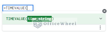
The time_string field holds the time representation. This field only takes a string value:

The time_string value can also be represented by a cell reference.

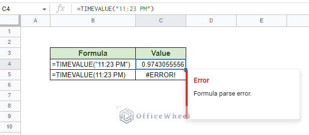
The most important thing to note is that the TIMEVALUE function sees the 24-hour day as a fraction, returning values between 0 (inclusive) and 1 (exclusive).

Here, the 0 value represents 12:00:00 AM and the 0.9999884259 represents 11:59:59 PM.

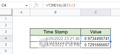
Note: When applying TIMEVALUE in cells that contain timestamps that include dates, the function will ignore the date portion:

Use of the TIMEVALUE Function in Google Sheets

Basic Example

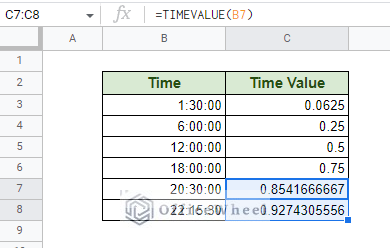
Here we have a simple table of dates in the 24-hour format and have applied the TIMEVALUE function for each of them:

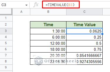
As you can see, as we move down the day, the time value increases. With 6:00:00 being the ¼ of a day, we get the corresponding 0.25 value. 0.5 for 12:00:00 and 0.75 for 18:00:00 or 6 PM and so on.

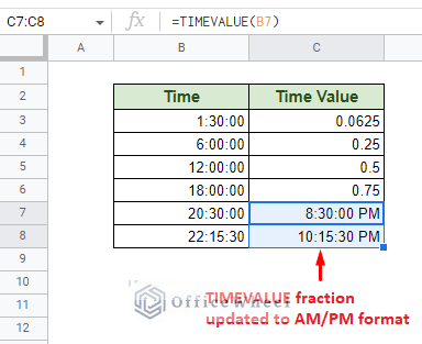
Now, we can also use a Time format for these values to return them to their corresponding times.

Step 1: Select the TIMEVALUE values you want to convert. We have chosen the last two values.

Step 2: Select the time format you want to convert this value to. We have navigated to the Time format (Time AM/PM) from the Format drop-down icon (123) from the Toolbar.

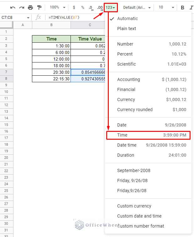
Step 3: Select the default time format to update the TIMEVALUE fraction to a proper time format. For us, it was the AM/PM time value.

Setting a Custom Time Format

Much like formatting custom dates, time formats can also be customized in Google Sheets according to the user’s needs.

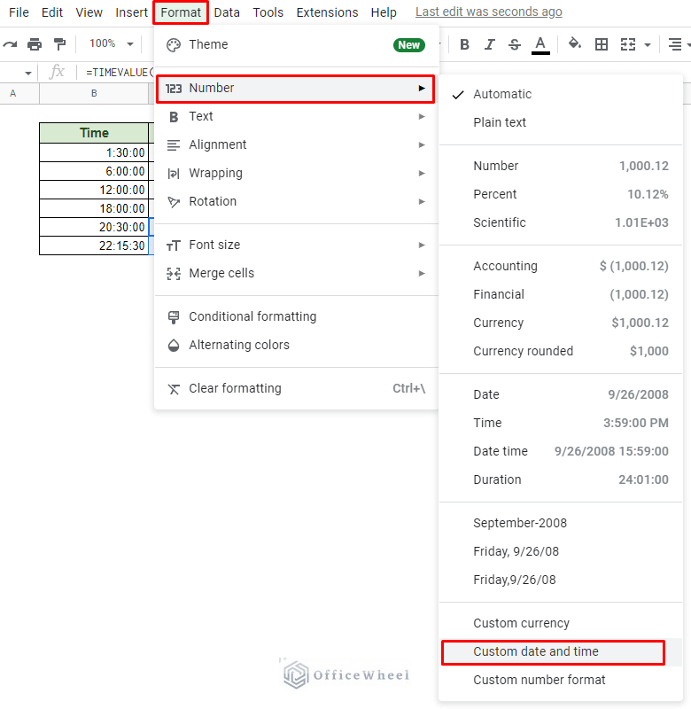
To set a custom time format, we need to first select a cell containing a time value (optional) and then navigate to the “Custom date and time” option from the Format tab.

Format > Number > Custom date and time

Now, in the Custom date and time formats window, we have a panel that contains how the current format of date or time is presented in our worksheet.

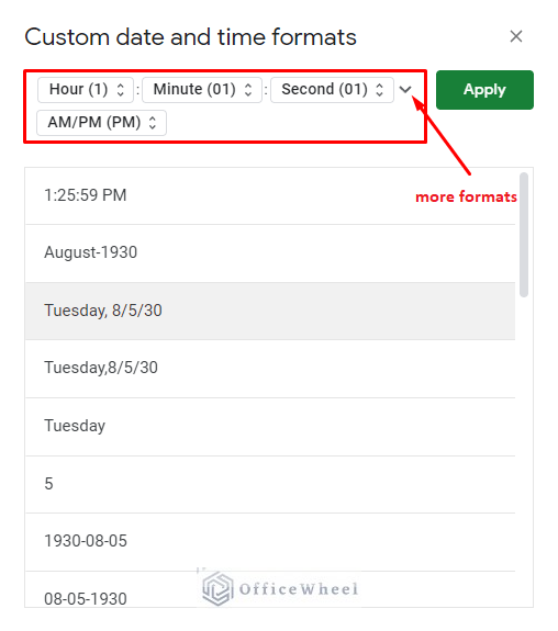
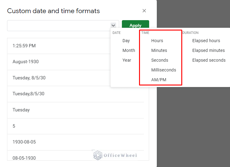
You can use the drop-down icon to see all the time options available. From here, you can choose the values you want to include in your time format and further customize them later.

Click Apply to apply the custom format on the selected cells.

Using TIMEVALUE for Different Time Formats in Google Sheets

As we have just seen, time can be presented in multiple different formats. But no matter the format, the underlying value remains the same. And that is what the TIMEVALUE function really uses.

Let’s have a look at some of the different but common time formats that can be seen in spreadsheets, and how the TIMEVALUE function reacts to them. Spoilers: There is little to no difference.

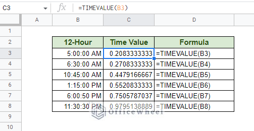
First up, we have the 24-hour time format in “HH:MM:SS” (Hours:Minutes:Seconds). This format is commonly used for the Arrival and Depart times for travel timetables.

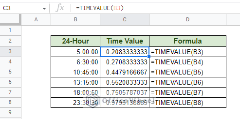
Next, we have the 12-hour day format where the entire day is split into two 12-hour sections. The time format looks like “HH:MM:SS AM/PM”. This format is most commonly used for daily entry and leave times for employees.

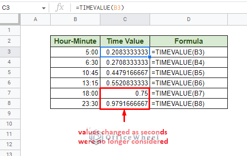
Another way of presenting time is the Hour-Minute format, “HH:MM”. The seconds time value is often not counted since any change in that value is minuscule. Here, we can see a slight change in the last two TIMEVALUE results as the seconds are not considered.

Finally, we have the Date-Time format, usually written as “MM/DD/YYYY HH:MM:SS”. This is the most data-heavy format for a cell. This is the default format of the NOW function.

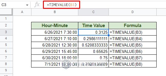
As you can see, TIMEVALUE ignores the date and only focuses on extracting the value of the time.

Example: Calculating Total Time Worked

One of the most common uses of time values is to calculate the time elapsed or time difference between two times.

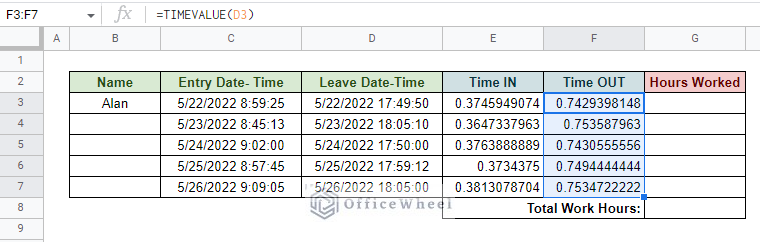
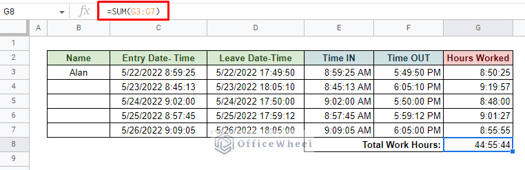
For our example, we have a sample dataset of an employee’s Entry and Leave timestamps for a week:

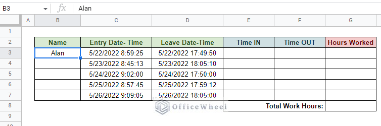
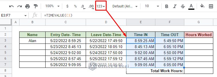
We are looking to retrieve only the time value from the Date-Time timestamp and present it in the 12-hour, HH:MM:SS AM/PM, format. Eventually, we want to calculate the total time elapsed from the newly found In and Out times. And also, optionally calculate the total hours worked in the week.

Here are the steps:

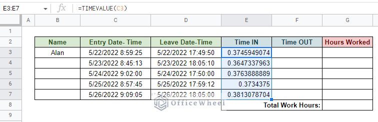
Step 1: Retrieve the IN time from the Entry Date-Time column with the TIMEVALUE function. Use the fill handle to apply the formula to the rest of the column.

Step 2: Retrieve the OUT time from the Leave Date-Time column with the TIMEVALUE function. Once again, use the fill handle down the column.

Step 3: Use simple formatting to convert these fractional time values in the Time IN and Time OUT columns to the 12-hour format.

Step 4: Use simple arithmetic subtraction between Time OUT and Time IN. This calculates the total hours worked.

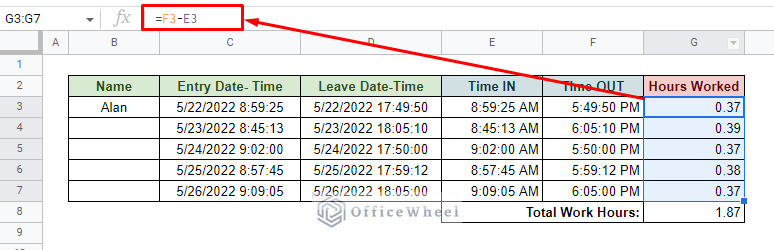
The calculated result may not be in the desired format. We will change that in the next step.

Step 5: Update the time format of the Hours Worked column, and subsequently the Total Hours Worked cell. From the Format toolbar option, we select Duration.

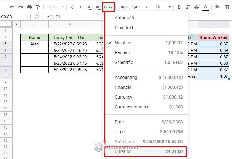
This results in the correct hours worked for each day. We have also used the SUM function to calculate the total.

Final Words

That concludes our simple guide to using the TIMEVALUE function in Google Sheets. It is a versatile function that can extract the value of time from any format to a fraction of 24 hours.

Feel free to leave any queries or advice you might have for us in the comments section below. Or have a look at some of our other articles that are sure to interest you.

Related Articles for Reading

• Find and Display Current Date in Google Sheets (Easy Guide)
• How to Use Today’s Date in Google Sheets (An Easy Guide)
• How to Convert Date to String in Google Sheets (An Easy Guide)
• Autofill Date when a Cell is Updated in Google Sheets (3 Easy Ways)
• How to Sum a Duration of Time in Google Sheets (An Easy Guide)