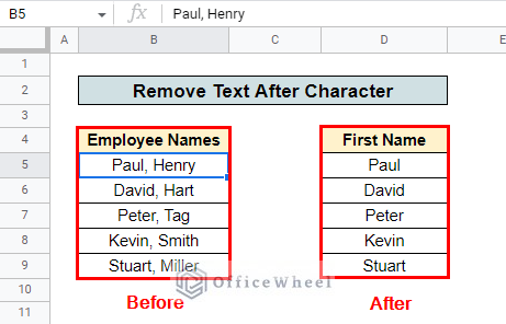
While working with texts in Google Sheets, there may come a situation when we need to remove certain text after a character or symbol. It can become very tiring and tedious to achieve this manually. Luckily, Google Sheets provides us with some easy ways to remove text after a character. In this article, we will learn how to remove text after a character in 5 methods.
A Sample of Practice Spreadsheet
5 Methods to Remove Text after Character in Google Sheets
1. Applying the Find and Replace Option
Find and Replace can be very useful to remove text after a character in Google Sheets. It is quite easy to apply.
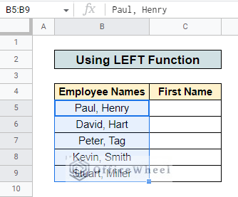
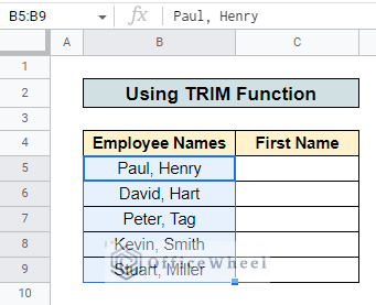
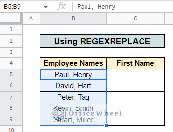
For this, you need to have a dataset first. We have a column with Employee Names on it in cells B5:B9. The first and last names are separated by a comma.
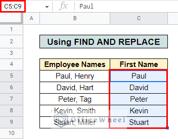
We want to get rid of the last names along with the comma and extract only the first names in cells C5:C9. These are the steps you need to follow:
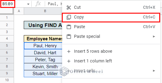
- First, Copy the table where the data is using the mouse or keyboard shortcut CTRL+C. In our example, we copy the B5:B9 table.
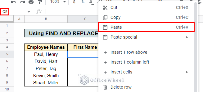
- Then Paste the whole table where you want the data table to appear. We want the first names to appear in cell C5 so we go to C5 and paste the table using CTRL+V.
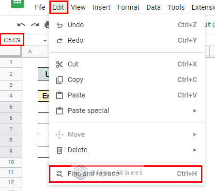
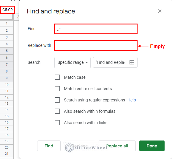
- Next, go to Edit > Find and replace or use CTRL+H on the keyboard to get the Find and replace popup.
- Now, In the popup window, type in ,.* in the Find box. Leave the Replace with box empty.
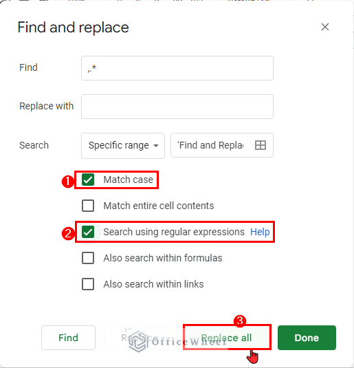
,.*- Then, check both Match case and Search using regular expressions and press Replace all.
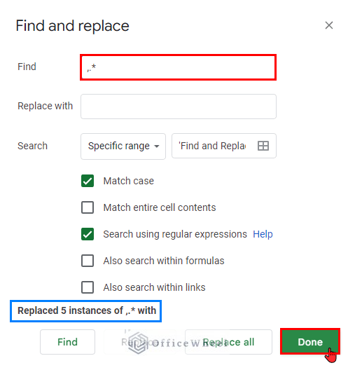
- Finally, press Done and only the first names of employees remain.
- Therefore, this is how you use Find and replace to remove text after a character in Google Sheets.
2. Using the LEFT and FIND Functions
The LEFT function can be used with the FIND function to remove text after a character in Google Sheets. It is one of the easier methods to learn. The LEFT function provides the substring from a cell containing a string starting from the left.
For this, you need to have a dataset first. For this, we have a column with Employee Names on it in cells B5:B9. We separate the first and last names by a comma.
We want to get rid of the last names along with the comma and show only the first names in cells C5:C9.
These are the steps you need to follow:
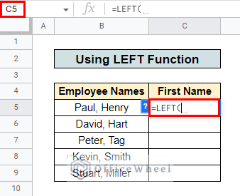
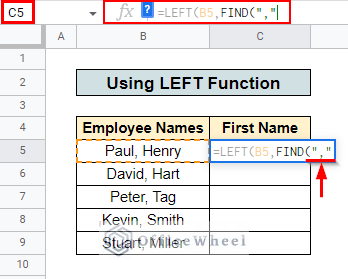
- First, go to the cell where you want the data to appear and type in
=LEFTfollowed by an opening parenthesis. In our example, We go to cell C5 and type in=LEFT(.
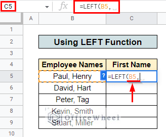
- Then, type in the cell number where the data is located followed by a comma. We type B5, as the data is in cell B5 in our table.
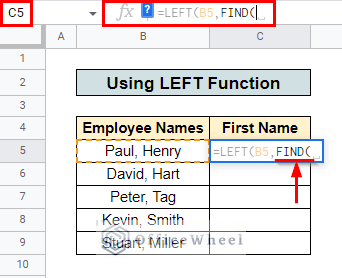
- Next, type in FIND followed by an opening parenthesis. We type in
FIND(.
- Now, as the data is separated by a comma, we type , inside a quotation. This means that data before the comma sign will appear in your new cell. So we type in “,”.
“,”
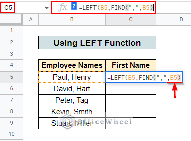
- Then, type in the cell name where the data is after a comma and close parentheses for the FIND function. In our case, we type in ,B5).
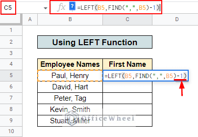
- Now, type -1, as you don’t want the comma to appear in your changed column, and close parentheses for LEFT function. In our example we type -1). This is what the final formula looks like:
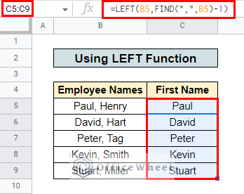
=LEFT(B5,FIND(",",B5)-1)- Finally, press ENTER and there you have a cell containing only the first portion of your data before a character. Copy this to the next columns and there you have your complete table.
Read More: How to Remove Last Character from String in Google Sheets
3. Applying TRIM Function with LEFT and FIND
TRIM function can be used along with LEFT and FIND functions to remove text after a character in Google Sheets.
Consider the dataset we had for the previous methods.
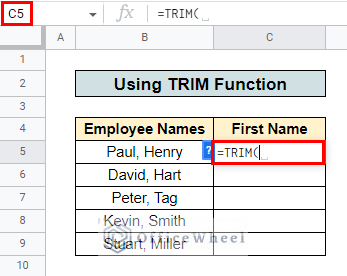
- First, go to the cell where you want the data to appear and type in
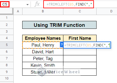
=TRIMfollowed by an opening parenthesis. In our example, We go to cell C5 and type in=TRIM(.
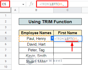
- Then, type in LEFT followed by an opening parenthesis. In our example, type in
LEFT(and type in the cell number where the data is, followed by a comma. We type B5, as the data is in cell B5 in our table.
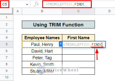
- Next, type in FIND followed by an opening parenthesis. We type in
FIND(.
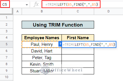
- Now, as the data is separated by a comma(,) we type , inside a quotation. This means that data before the comma sign will appear in your new cell. So we type in
“,”.
- Then, type in the cell name where the data is after a comma and close parentheses for the FIND function. In our case, we type in
,B5).
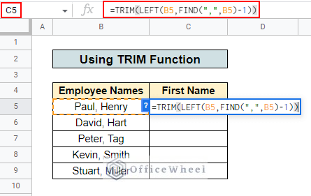
- Now, type -1, as you don’t want the comma to appear in your changed column and close parentheses for the LEFT function and as well as for the TRIM function. In our example we type
-1)). This is how the final formula looks:
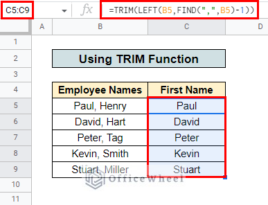
=TRIM(LEFT(B5,FIND(",",B5)-1))- Finally, Press ENTER, and there you have a cell containing only the first portion of your data before a character. Copy this to the next columns and there you have your complete table.
Read More: Remove Everything after Character Using Google Sheets Formula
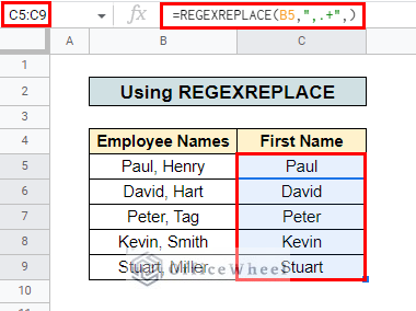
4. Remove Text with the REGEXREPLACE Function
REGEXREPLACE function can be used to remove text after a character in Google Sheets. It can be implemented in the following ways:
Consider the dataset we used for the above methods.
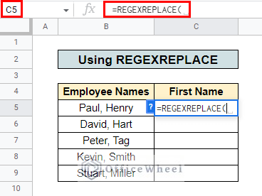
- First, go to the cell where you want to show the data and type
=REGEXREPLACEfollowed by an opening parenthesis. For our example, we go to cell C5 and type=REGEXREPLACE(.
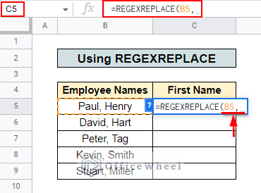
- Then, type in the cell number where the data is currently located followed by a comma. In our example, as the data is in cell B5 we type B5,.
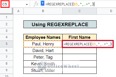
- Now, type ,.+ inside a quotation as we want to replace the data after the comma. Then, type in a comma and close parentheses. So, we type
",.+",).
",.+"- Therefore, this is how the final formula looks:
=REGEXREPLACE(B5,",.+",)- Finally, Press ENTER, and there you have a cell containing only the first portion of your data before a character. Copy this to the next columns and there you have your complete table.
5. Using the REGEXEXTRACT Function
REGEXEXTRACT can also be used to remove text after character in Google Sheets. Just follow the following steps:
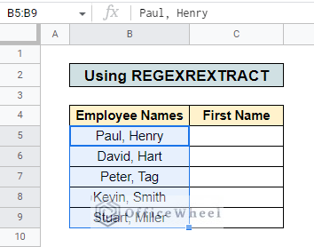
Consider the dataset we used for the above methods.
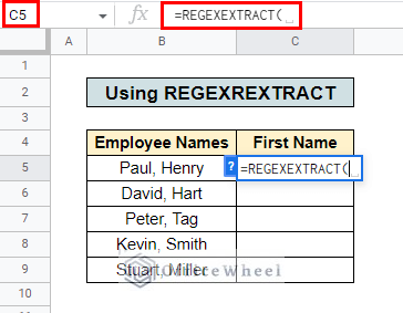
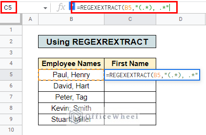
- First, go to the cell where you want to show the data and type
=REGEXEXTRACTfollowed by an opening parenthesis. For our example, we go to cell C5 and type=REGEXEXTRACT.
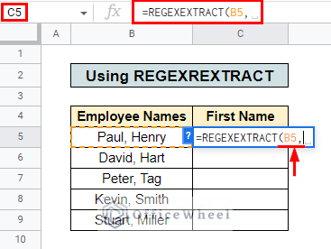
- Then, you type in the cell number where the data currently is located. Then type a comma. In our example we type B5,.
- Now, type (.*) starting a quotation as we want to show this data. In our example, we type “(.*).
- Then, type in COMMA SPACE and .* and close the quotation. We type in , .*” as we do not want to show anything after the comma.
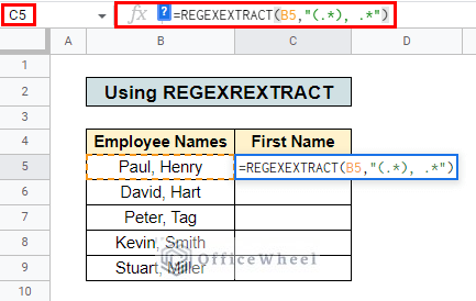
"(.*), .*"- Then close parentheses for REGEXEXTRACT. This is how the final formula looks:
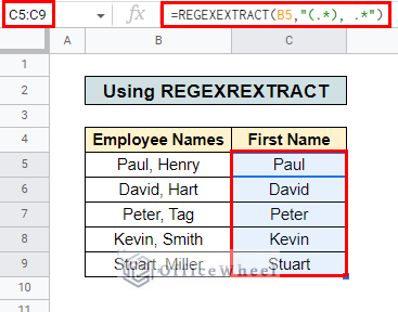
=REGEXEXTRACT(B5,"(.*), .*")- Finally, Press ENTER, and there you have a cell containing only the first portion of your data before a character. Copy this to the next columns and there you have your complete table.
Read More: How to Remove First Character in Google Sheets
Conclusion
In this article, we showed you how to remove text after a character in Google Sheets. We hope this article was useful to you. Keep on practicing the 5 methods that were shown here to get a grip on the concept.
Also, check out our other articles on OfficeWheel to keep on improving your Google Sheets work knowledge.

