In Google Sheets, if you want to count values except for any specific values, you can also apply the COUNTIF function with a specialized operator. The “<>” operator stands for “Not Equal”. In this article, we will explain about the Google Sheets COUNTIF function for cells not equal to text.
A Sample of Practice Spreadsheet
You can download the practice spreadsheet from the download button below.
3 Examples to Use COUNTIF for Cells Not Equal to Text in Google Sheets
You can use this COUNTIF function for calls not equal to text in three ways.
COUNTIF syntax:
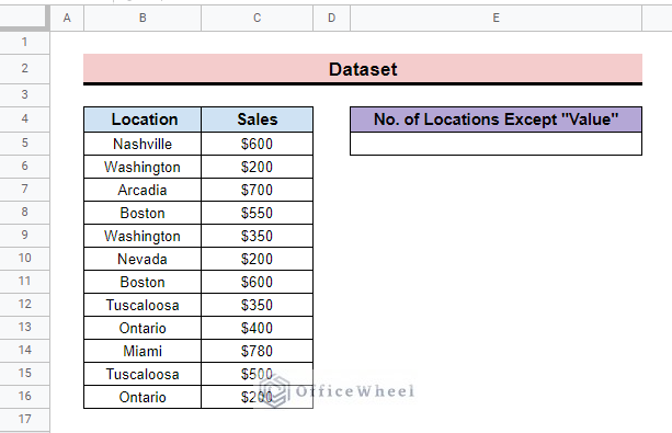
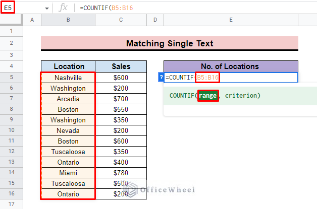
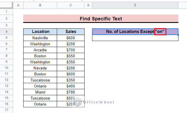
=COUNTIF(range, criterion)To apply the methods here we develop a dataset representing the Location and Sales. From where you can count values by skipping any one or more values. We have a total of 12 data rows here.
Here, we also create a column where you can insert specific values to run the function.
1. COUNTIF Cells Are Not Equal to Specific Text
It is the simplest way to use the COUNTIF not equal to a single text. In this method, you have to insert a specific text in the function COUNTIF, and it returns the total column count except for the number of the specific value. To do so,
Steps:
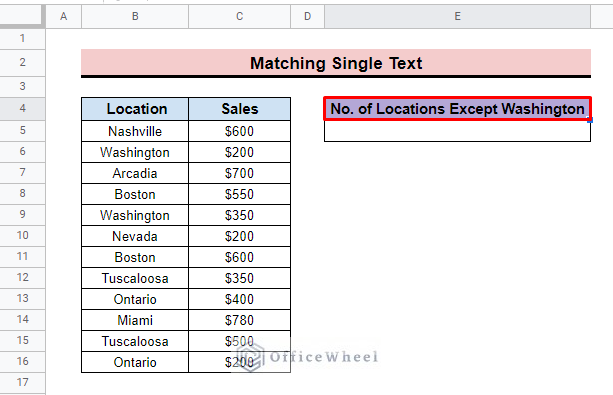
- In the beginning, select a value and add it to the function applied title. Here we add ‘Washington’ as a specific value.
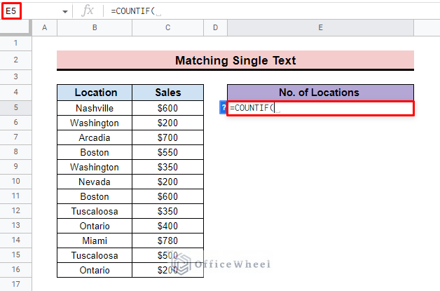
- After that select cell E5 and insert the COUNTIF function in the cell.
- Now, in the function for the range argument add the entire Location column with the B5:B16 cell range.
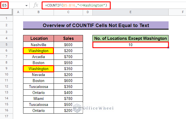
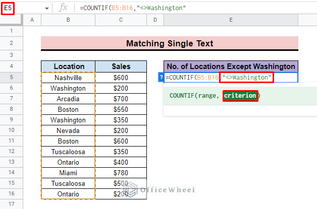
- For criteria parameter input ”<>Washington” in the function. Here, <> is for ‘Not Equal’ and “Washington” is the specific value.
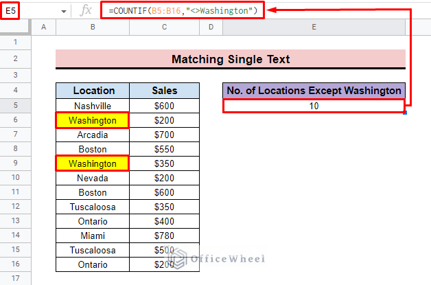
- Finally, press ENTER, and you will find the count of values which does not contain the value” Washington”.
=COUNTIF(B5:B16,”<>Washington”)Read More: Use COUNTIF If Cell Contains Specific Text in Google Sheets
2. Count Cells That Do Not Contain Any Text
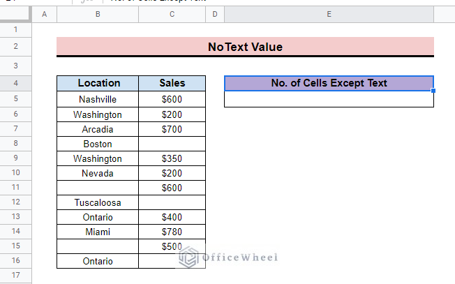
You can also use the COUNTIF function to count cells not containing any text. To Apply the example we use a dataset that contains blank cells also. Here, we consider the blank and numeric cells except for text cells.
Steps:
- First, create a dataset that contains blank cells along with numeric and text cells.
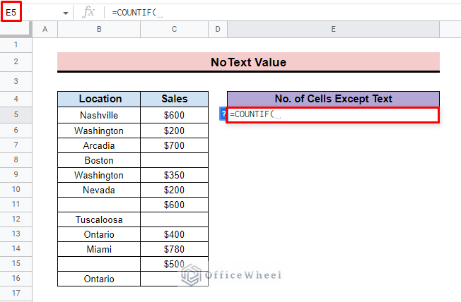
- Then select cell E5 and insert the COUNTIF function.
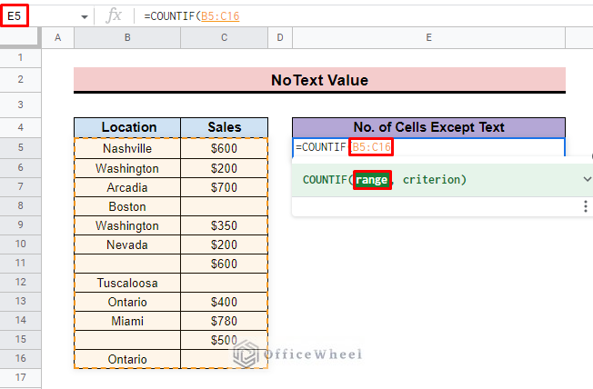
- After that input the entire dataset as a range.
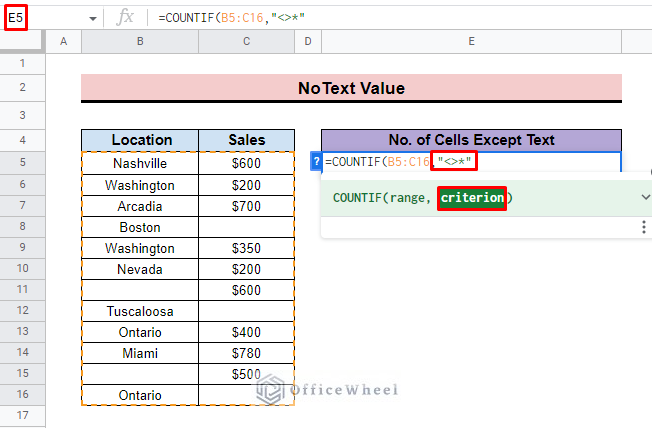
- Now add “ <>* ” as the second argument.
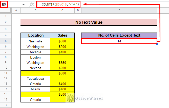
- Finally, press ENTER, and you will find the count of cells skipping the text value. Here, the function counts the numeric and blank cells.
=COUNTIF(B5:B16,"<>*")Read More: COUNTIF Function with “Not Equal to” Criterion in Google Sheets
Similar Readings
- How to Use COUNTIF Function with OR Logic in Google Sheets
- COUNTIF with Greater than and Less than Criteria in Google Sheets
- How to Use VLOOKUP with COUNTIF Function in Google Sheets
3. Tally for Cells Without Partial Text Match
For searching any partial text, the asterisk (*) wildcard is very useful. You can use this symbol for the COUNTIF not equal to the text formula if you insert a partial text and want to count except that value. To do so,
Steps:
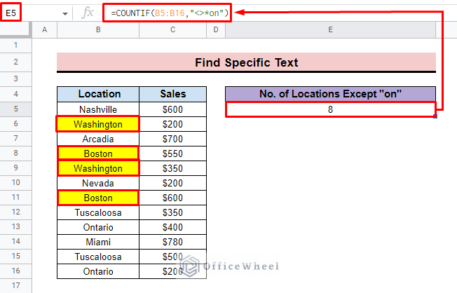
- First, we create the result column where we count values except those that end with “on”.
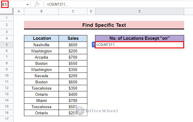
- Then select cell E5 and insert the COUNTIF function.
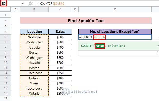
- After that add B5:B16 as the range of the function.
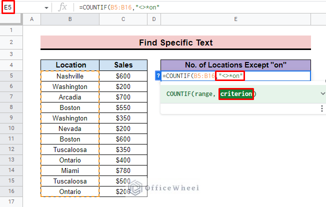
- Then input the criterion “<>*on” in the function. Here, <> represents the Not Equal, and *on represents all the values that end with “on” text.
- Finally, click on ENTER to apply the formula and you will find the desired result.
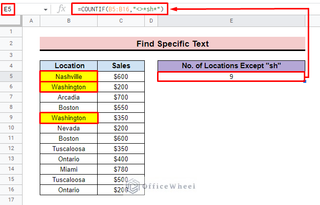
=COUNTIF(B5:B16,”<>*on”)- Similarly, you can apply the same process for a middle partial text. Here, we add a partial test “sh” which is a middle portion of the exact text in the dataset.
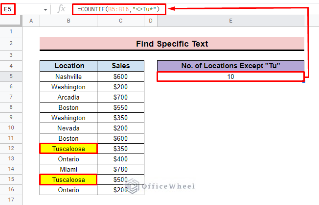
=COUNTIF(B5:B16,”<>*sh*)- Additionally, for beginning partial text the same methods can be applied. Here, we add “Tu” as the beginning partial text.
=COUNTIF(B5:B16,”<>Tu*”)Read More: [Fixed!] COUNTIF Function Is Not Working in Google Sheets
How to Use COUNTIFS If Cells Are Not Equal to Multiple Texts in Google Sheets
You can also apply the function if you want to count by ignoring two or more values. For executing this method, we have to use the COUNTIFS function instead of COUNTIF.
Steps:
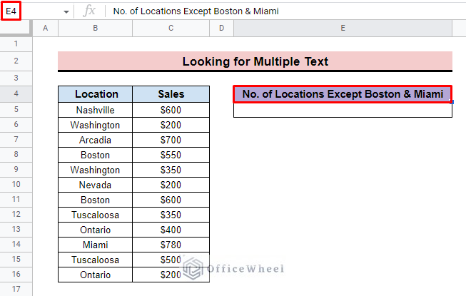
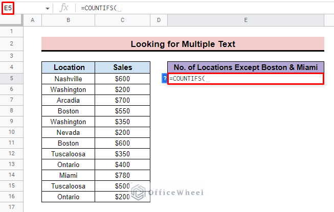
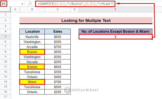
- In the first step, create a result column name “No. of Locations Except Boston & Miami” where you apply the formula.
- Then select cell E5 and insert the COUNTIFS function.
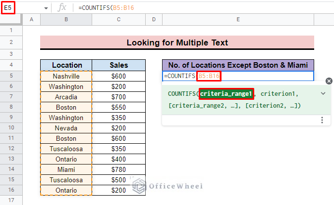
- Now add the entire Location column range B5:B16 as criteria_range1 argument.
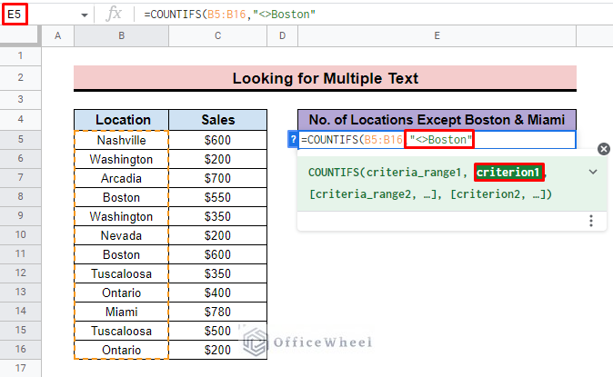
- After that, input “<>Boston” as the criterion1 parameter.
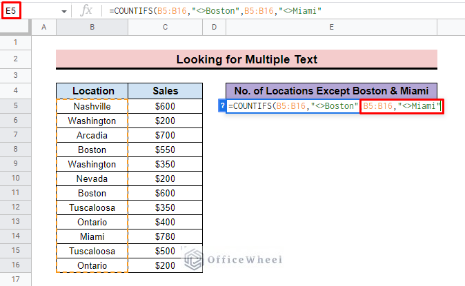
- In the same way, we add another range and criterion for “Miami”. You can add as many values as you want by following the same process.
- Finally, press ENTER, and you will find the count number except for Boston and Miami.
- As these two texts are placed in three times so the count number is 9 instead of the total count value of 12.
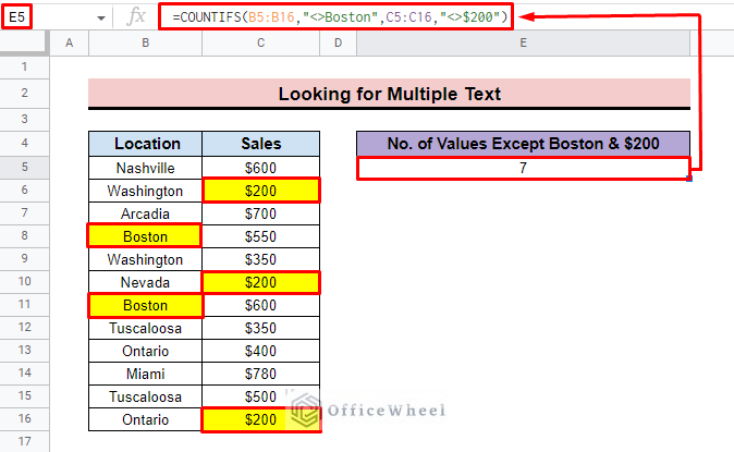
- Additionally, you can also apply the same method for different column ranges and extract the final value. Here we count the number of values except for Boston and $200 and we get the result 7.
=COUNTIF(B5:B16,"<>Boston",C5:C16,"<>$200)Read More: Google Sheets Count Cells from Another Workbook with COUNTIF Function
Things to Remember
- Always be careful about inserting text as the function is case-sensitive.
- Properly insert the range in the function.
Conclusion
After going through the article, we believe you can build a clear concept about how to use COUNTIF for cells not equal to text in Google Sheets. To explore more about Google Sheets, you can visit the OfficeWheel website.

