Google Sheets: Convert Time to Number (3 Easy Ways)

This article will look at how to convert time to a number value in Google Sheets. It can be in hours, minutes, or seconds in decimal form.

Fundamentally, while date and time are seen as numerical values in Google Sheets, they are special in the sense that they are presented in a different format which can affect calculations.

This is the primary reason why we’d want to convert a time value to decimals. Other reasons may include presenting time in a different format due to requirements, like calculating the total number of minutes elapsed for one.

Let’s see how it’s done.

3 Ways to Convert Time to a Number in Google Sheets

1. Using Time Functions like HOUR, MINUTE, and SECOND to Convert Time to a Number

Google Sheets already has some great time functions designed for us. They are the HOUR, MINUTE, and SECOND functions.

Let’s see how they work with a simple example.

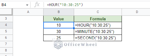
Consider the time 10:30:25. This is in the HH:MM:SS format, where H is hours, M is minutes, and S is seconds.

Each of the previously mentioned functions will extract their respective values from this time.

Applying the HOUR function will give us 10:

The MINUTE function will give us 30:

And the SECOND function will give us 25:

With these three functions, we have successfully split a time value in Google Sheets into its respective hours, minutes, and seconds.

All that remains is to use these values in simple calculations to get the number values that we are looking for.

Convert Time to Hours Passed

To convert an entire time value to one of its sub-values, we must convert all of the sub-values into one type.

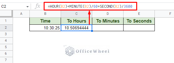
For example, to convert a time to only hours, we must take the hour value and convert the minute and second values to hours. And finally, sum them together

To convert 10:30:25 to hours:

1. The HOUR function remains the same:

2. Converting minutes to hours:

Since there are 60 minutes to an hour, we divide the value by 60.

3. Converting seconds to hours:

Since there are 3600 seconds to an hour (60*60), we divide the value by 3600.

Adding them all together with cell reference:

Convert Time to Minutes Passed

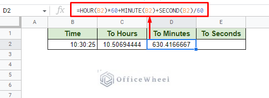
Converting time to decimal minutes follows the same idea for converting time to hours: convert and add. Only this time, the value will be in minutes.

1. Converting hours to minutes:

2. Keep the minute value unchanged:

3. Convert seconds to minutes:

Adding them all together with cell reference:

Convert Time to Decimal Seconds

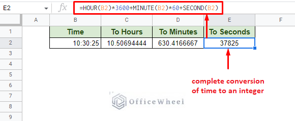
Finally, we come to the conversion of time to seconds. With seconds being the smallest version of time, the result will be the true conversion of time to an integer number.

The conversion formula itself is the direct opposite of the hour conversion.

1. Converting hours to seconds:

2. Converting minutes to seconds:

3. Leave the seconds value as it is:

Adding them all together with cell reference:

This method also shows how to convert time to an integer number or decimals in Google Sheets.

2. Using the TIMEVALUE Function to Convert Time to a Number in Google Sheets

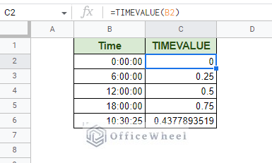
TIMEVALUE is a unique time function in Google Sheets that returns a time value as a fraction of a day or 24 hours.

So, passing 12:00:00 through the TIMEVALUE function will give us 0.5 since it is half of a day. We will get 0.25 for 6:00:00 and 0.75 for 18:00:00. You get the idea.

To get the hour, minute, and second values from the TIMEVALUE results, we must simply multiply them by the respective hour, minute, and second values equivalent to a single day.

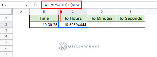
For example, to convert time to decimal hours with TIMEVALUE, we must multiply it by 24. Since there are 24 hours to a day:

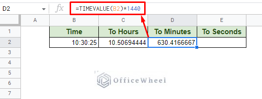
To get the number of minutes, we must multiply it by 1440 (24 hours * 60 minutes):

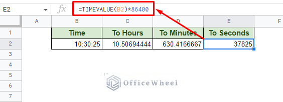
Finally, to get the number of seconds from time, we must multiply by 86400 (24 hours * 60 minutes * 60 seconds)

3. Using the Convert Function to Convert Time to a Number in Google Sheets

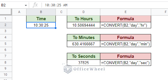
CONVERT is another function that we can use to convert time to a number in Google Sheets.

While it is a more general function used to convert one similar value to another, it can be easily applied to time calculations.

In this case, the “value” field will be covered by the time.

The “start_unit” field will have the “day” value since we will be considering the entire day as a unit (you can also use “d”). Much like what we’ve seen with the TIMEVALUE method.

Finally, the “end_unit” will be covered by the required number value:

• “hr”: Hours
• “min” or “mn”: Minutes
• “sec” or “s”: Seconds

So, the corresponding formulas are:

Final Words

That concludes the three ways we can use to convert time to a number in Google Sheets.

It is all about extracting each sub-value of time and converting them. Or by converting a time value to a day and applying simple multiplication.

Google Sheets makes these approaches that much easier by providing us with great time functions, of which, one of my favorites is the TIMEVALUE function.

Feel free to leave any queries or advice you might have for us in the comments section below.

Related Articles for Reading

• How to Change a Number Format in Google Sheets (An Easy Guide)
• Format a Number with a Formula in Google Sheets
• How to Format Numbers as Text in Google Sheets (5 Easy Examples)
• How to Insert a Timestamp in Google Sheets (An Easy Guide)