The AVERAGEIFS function is similar to the AVERAGEIF function, except for the fact that the AVERAGEIFS function can deal with multiple mutually inclusive criteria whereas the AVERAGEIF function can only deal with a single criterion. The statistical function AVERAGEIFS often uses criteria from two different columns since data from a single column that meets multiple criteria is rarely mutually inclusive. So how to use the AVERAGEIFS function with multiple criteria in the same column in Google Sheets? Despite being a rare scenario, we can show you 2 helpful examples. Keep reading to learn the examples.
A Sample of Practice Spreadsheet
You can download a sample of the practice spreadsheet by clicking on the following link. The spreadsheet consists of an overview of the datasheet and an outline of the described ways for using the AVERAGEIFS function with multiple criteria in the same column.
What Is AVERAGEIFS Function in Google Sheets?
The AVERAGEIFS function is used for returning the average of a range of numbers depending on multiple criteria.
Syntax
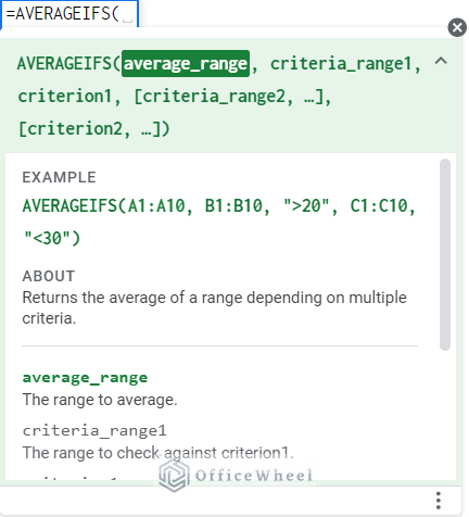
The syntax of the function is following:
AVERAGEIFS(average_range, criteria_range1, criterion1, [criteria_range2, …], [criterion2, …])Arguments
The arguments of the AVERAGEIFS function are the following:
| Arguments | Requirement | Function |
|---|---|---|
| average_range | Required | The range for which you want to determine the average |
| criteria_range1 | Required | The range you want to be checked for criterion1 |
| criterion1 | Required | The condition that you want to be applied to criteria_range1 |
| criteria_range2, … | Optional | Repeatable additional ranges to check |
| criterion2, … | Optional | Repeatable additional criteria to check |
Output
The formula =AVERAGEIFS(E5:E14,D5:D14,”>30″,C5:C14,”Single”) will find the average of selective cells in range E5:E14 by following two criteria: subsequent value in Column D has to be greater than 30 and subsequent text in Column C has to be “Single”.
2 Helpful Examples of Using AVERAGEIFS Function with Multiple Criteria in Same Column in Google Sheets
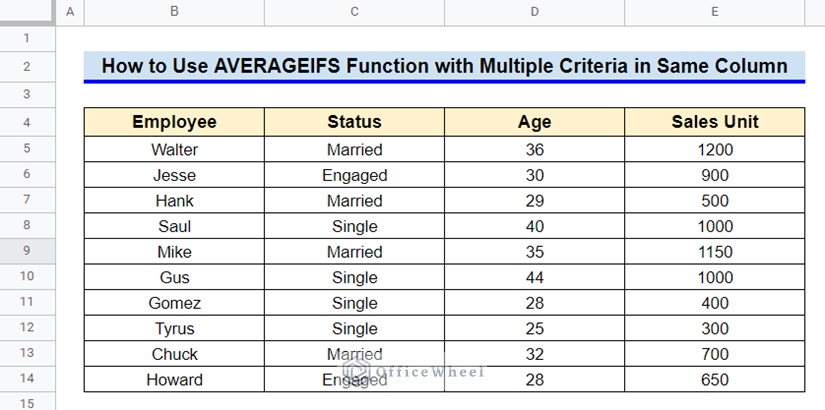
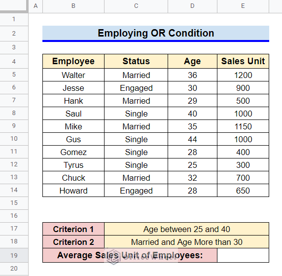
First, let’s get familiar with our datasheet. It consists of several employees’ Names, Statuses, Ages, and Sales Unit data. We’ll use multiple criteria from a single column to calculate average sales.
1. Dealing with Logical Operators
Logical operators are symbols or words that connect two or more expressions. Three logical operators are mostly used: AND, OR, and NOT. In AVERAGEIFS function, the criteria are typically mutually inclusive. So, we will use AND condition here.
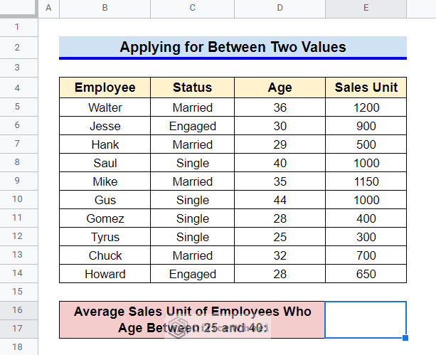
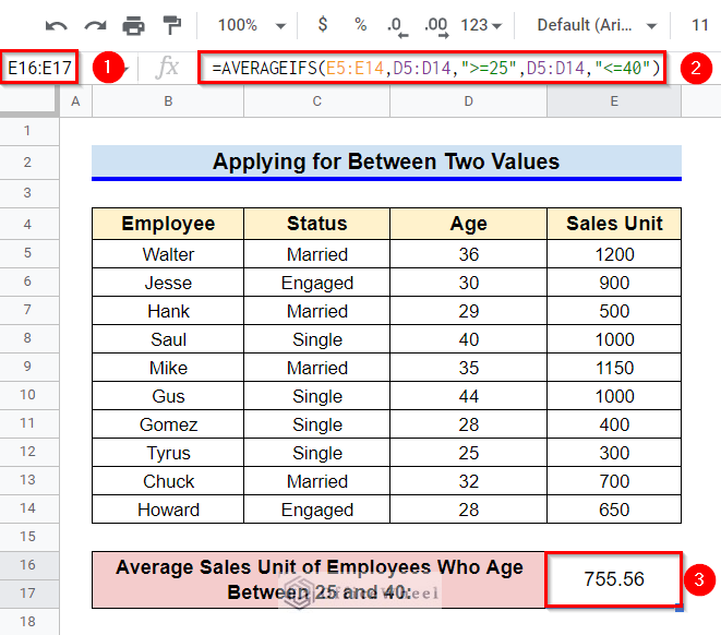
Since, we will take our criteria from a single column, only “between two values” criteria will be mutually inclusive. So, let’s calculate the average sales unit of employees aged between 25 and 40.
Steps:
- First, modify your datasheet like the following.
- Then, select the cell where you want to calculate the average and type in the following formula-
=AVERAGEIFS(E5:E14,D5:D14,">=25",D5:D14,"<=40")- Finally, press Enter key to get the required average value.
Read More: How to Use AVERAGEIFS Function Between Two Times in Google Sheets
2. Employing for OR Condition
Is it possible to employ an OR condition while using the AVERAGEIFS function even though that goes against the structure of the arguments of the AVERAGEIFS function? Yes, it is possible if you apply some techniques. We are going to use multiple AVERAGEIFS functions for this operation.
First, let’s assume our criteria for applying OR condition in the AVERAGEIFS function:
Criterion 1: Age between 25 and 40.
Criterion 2: Married and Age More than 30.
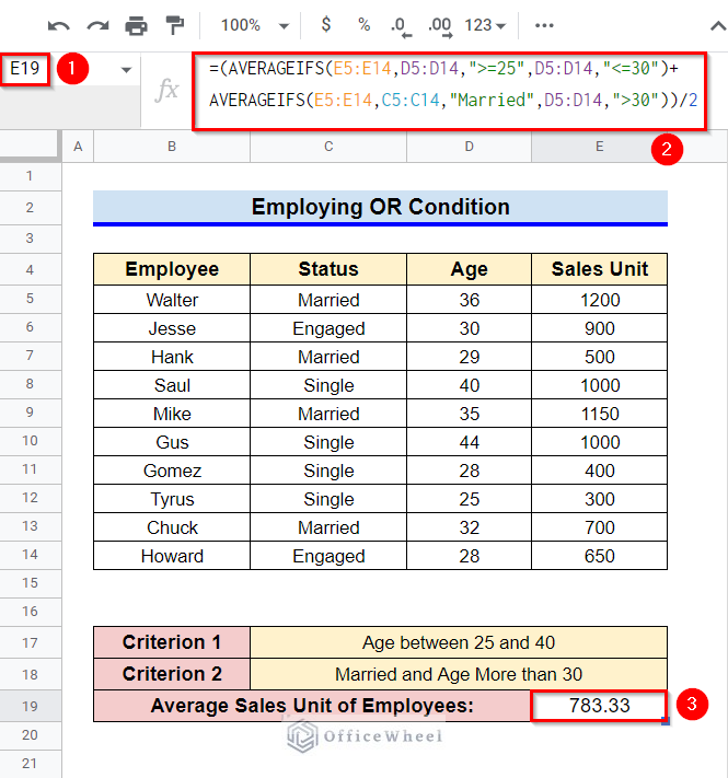
Now, let’s calculate the average sales unit of employees who follow either Criterion 1 or Criterion 2.
Steps:
- Firstly, modify your datasheet like the following.
- Then, select Cell E19 and type in the following formula-
=(AVERAGEIFS(E5:E14,D5:D14,">=25",D5:D14,"<=30") +AVERAGEIFS(E5:E14,C5:C14,"Married",D5:D14,">30"))/2- Finally, after pressing the Enter key, we’ll get the average for the sales units which meet our criteria.
Formula Breakdown
- AVERAGEIFS(E5:E14,C5:C14,”Married”,D5:D14,”>30″)
First, this AVERAGEIFS function calculates the average sales unit of employees in the range E5:E14 if any match is found for the criterion “Married” in the range C5:C14 and “>30” in the range D5:D14.
- AVERAGEIFS(E5:E14,D5:D14,”>=25″,D5:D14,”<=30″)
Similarly, the other AVERAGEIFS function calculates the average sales unit of employees in the range E5:E14 if the values in the range D5:D14 are between 25 and 30.
- (AVERAGEIFS(E5:E14,D5:D14,”>=25″,D5:D14,”<=30″)+ AVERAGEIFS(E5:E14,C5:C14,”Married”,D5:D14,”>30″))/2
Finally, the returned values from the AVERAGEIFS functions are added and then divided by 2 to get the required result.
Read More: How to Average If Cells Have Multiple Conditions in Google Sheets
Things to Be Considered
- The criteria used in the AVERAGEIFS function have to be mutually inclusive. Else, you will get a division by zero error.
- While employing the OR condition in the AVERAGEIFS function, in the end, remember to divide by the number of times the AVERAGEIFS functions are used.
- The range of the argument average_range has to be equal while employing the OR condition using the AVERAGEIFS function.
Conclusion
This concludes our article to learn how to use the AVERAGEIFS function with multiple criteria in the same column in Google Sheets. Although very few examples can be provided with these conditions, I hope that the mentioned examples will be sufficient for your requirement. Feel free to share your comments and advice in the comment box.

